Basis

import matplotlib.pyplot as plt
import numpy as np
import sympy as sy

sy.init_printing()

import linear_algebra_visulization

Basis, denoted as \(B\), is the minimum unit of user-customized coordinates, which is any type of coordinate system other than Cartesian.

Basis of \(\mathbb{R}^2\)

Formally speaking, the basis is a set of vectors \(B\) in vector space \(V\) with two conditions: 1. All vectors in \(B\) are independent. 2. \(\text{span}(B)=V\)

We have seen standard basis in earlier chapters, for instance in \(\mathbb{R}^2\)

\[e_1= \left[ \begin{matrix} 1\\0 \end{matrix} \right], \ e_2=\left[ \begin{matrix} 0\\1 \end{matrix} \right] \]

and in \(\mathbb{R}^3\)

\[e_1= \left[ \begin{matrix} 1\\0\\0 \end{matrix} \right], \ e_2=\left[ \begin{matrix} 0\\1\\0 \end{matrix} \right], \ e_3=\left[ \begin{matrix} 0\\0\\1 \end{matrix} \right] \]

Here we show the linear combination of standard basis for vector \((3, 6)\)

fig, ax = plt.subplots(figsize=(10, 10))

arrows = np.array(
    [[[0, 0, 1, 0]], [[0, 0, 0, 1]], [[0, 0, 3, 0]], [[0, 0, 0, 6]], [[0, 0, 3, 6]]]
)

colors = ["r", "b", "r", "b", "g"]
for i in range(arrows.shape[0]):
    X, Y, U, V = zip(*arrows[i, :, :])
    ax.arrow(
        X[0],
        Y[0],
        U[0],
        V[0],
        color=colors[i],
        width=0.03,
        length_includes_head=True,
        head_width=0.2,  # default: 3*width
        head_length=0.3,
        overhang=0.4,
    )

############################Dashed##################################
line1 = np.array([[3, 0], [3, 6]])
ax.plot(line1[:, 0], line1[:, 1], ls="--", lw=3, color="black", alpha=0.5)

line2 = np.array([[0, 6], [3, 6]])
ax.plot(line2[:, 0], line2[:, 1], ls="--", lw=3, color="black", alpha=0.5)

############################Text#####################################

ax.text(0, 1, "$e_2$", size=15)
ax.text(1, 0, "$e_1$", size=15)

ax.text(0, 6, "$6e_2$", size=15)
ax.text(3, 0, "$3e_1$", size=15)

ax.text(3, 6, "$3e_1+6e_2$", size=15)

###########################Grid Setting##############################
# Major ticks every 20, minor ticks every 5
major_ticks = np.arange(0, 10, 2)
minor_ticks = np.arange(0, 10, 0.5)

ax.set_xticks(major_ticks)
ax.set_xticks(minor_ticks, minor=True)

ax.set_yticks(major_ticks)
ax.set_yticks(minor_ticks, minor=True)

ax.grid(which="both")
ax.grid(which="minor", alpha=0.2)
ax.grid(which="major", alpha=0.5)

#######################################################################
ax.set_xlabel("x-axis", size=18)
ax.set_ylabel("y-axis", size=18)
ax.axis([-1, 10, -1, 10])
ax.grid()
plt.show()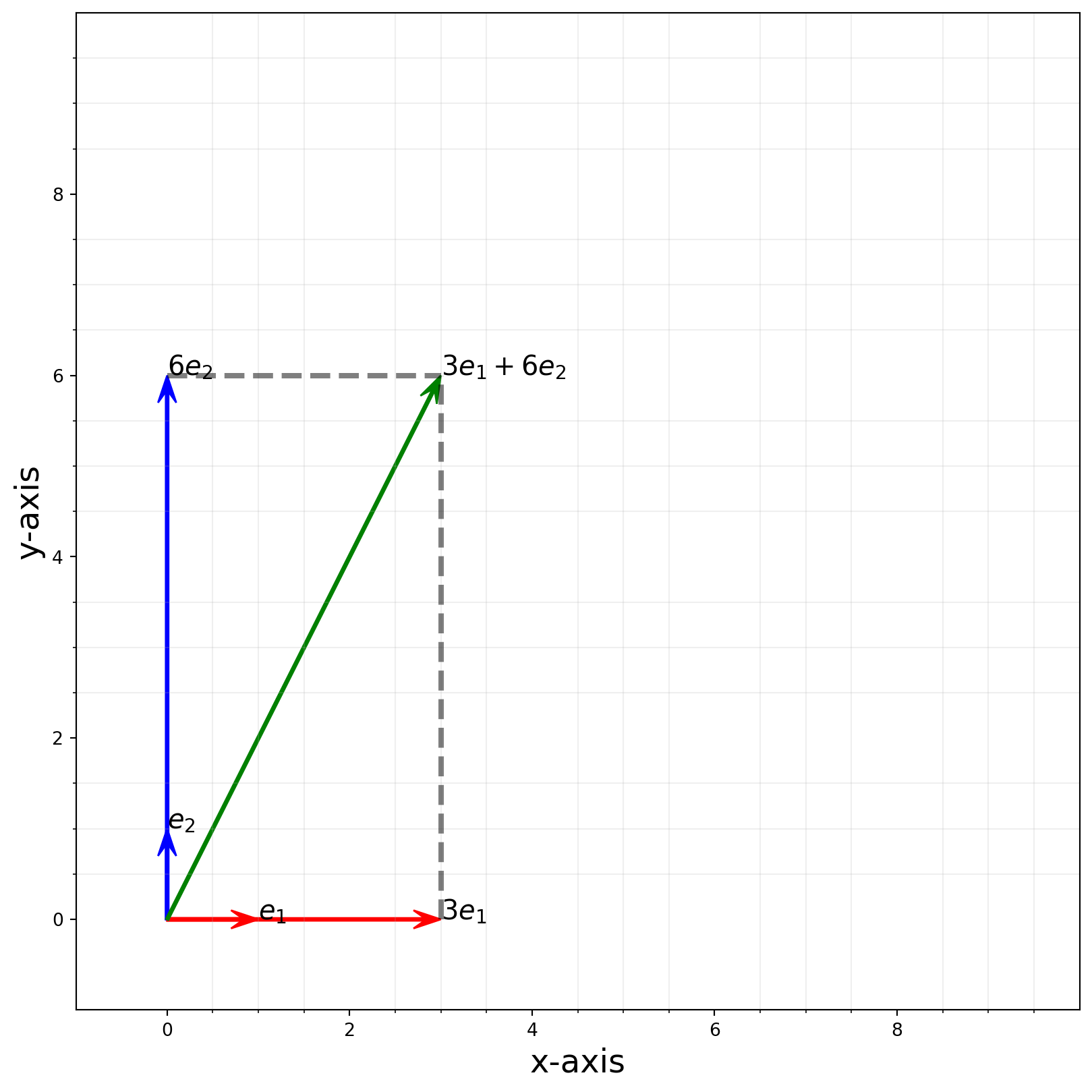

But non-standard basis is what we mostly use, we can show that \((2, 1)\) and \((-1, 2)\) is a basis for \(\mathbb{R}^2\).

fig, ax = plt.subplots(figsize=(10, 10))

v1 = np.array([2, 1])
v2 = np.array([-1, 2])
v1m2 = 2 * v1
v2m3 = 3 * v2

arrows = np.array(
    [
        [[0, 0, v1[0], v1[1]]],
        [[0, 0, v2[0], v2[1]]],
        [[0, 0, 2 * v1[0], 2 * v1[1]]],
        [[0, 0, 3 * v2[0], 3 * v2[1]]],
        [[0, 0, (v1m2 + v2m3)[0], (v1m2 + v2m3)[1]]],
    ]
)

colors = ["r", "b", "r", "b", "g"]
for i in range(arrows.shape[0]):
    X, Y, U, V = zip(*arrows[i, :, :])
    ax.arrow(
        X[0],
        Y[0],
        U[0],
        V[0],
        color=colors[i],
        width=0.03,
        length_includes_head=True,
        head_width=0.2,  # default: 3*width
        head_length=0.3,
        overhang=0.4,
    )

# ############################ Dashed ##################################

point1 = [v2m3[0], v2m3[1]]
point2 = [v2m3[0] + v1m2[0], v2m3[1] + v1m2[1]]
line = np.array([point1, point2])
ax.plot(line[:, 0], line[:, 1], ls="--", lw=3, color="black", alpha=0.5)

point1 = [v1m2[0], v1m2[1]]
point2 = [v2m3[0] + v1m2[0], v2m3[1] + v1m2[1]]
line = np.array([point1, point2])
ax.plot(line[:, 0], line[:, 1], ls="--", lw=3, color="black", alpha=0.5)

############################Text#####################################

ax.text(2, 1, "$v_1$", size=15)
ax.text(-1, 2, "$v_2$", size=15)

ax.text(v1m2[0], v1m2[1], "$2v_1$", size=15)
ax.text(v2m3[0], v2m3[1], "$3v_2$", size=15)

ax.text(v1m2[0] + v2m3[0], v1m2[1] + v2m3[1], "$2v_1+3v_2$", size=15)
############################## Grid ###############################

t = np.linspace(-6, 6)
for k in range(-6, 7):
    x = 2 * k - t
    y = k + 2 * t
    ax.plot(x, y, ls="--", color="red", alpha=0.3)

for k in range(-6, 7):
    x = -k + 2 * t
    y = 2 * k + t
    ax.plot(x, y, ls="--", color="red", alpha=0.3)

#######################################################################
ax.set_xlabel("x-axis", size=18)
ax.set_ylabel("y-axis", size=18)
ax.axis([-6, 6, 0, 10])  # np.linalg.norm(v1m2+v2m3) is intercept
plt.show()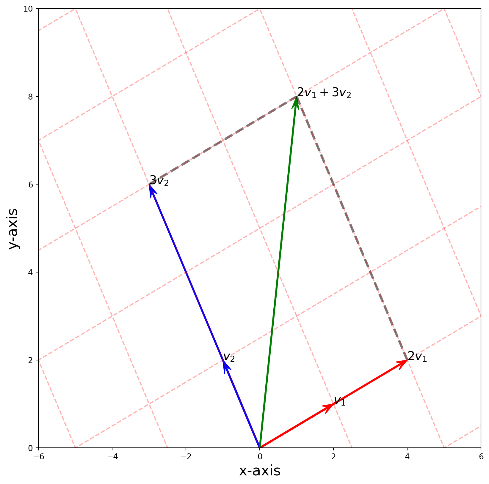

Whether basis is standard or not, as long as they are independent, they span \(\mathbb{R}^2\).

Basis of \(\mathbb{R}^3\)

Next we show the standard basis and a non-standard basis of \(\mathbb{R}^3\).

The standard basis in \(\mathbb{R}^3\) is

\[ (e_1, e_2, e_3)= \left[ \begin{matrix} 1 & 0 & 0\\ 0 & 1 & 0\\ 0 & 0 & 1 \end{matrix} \right] \]

and we can show a vector \((2,3,4)\) in \(\mathbb{R}^3\) is a linear combination of them. We did a 3D linear combination plot in lecture 6, here we just reproduce it by importing the module at the top of the note.

linear_algebra_visulization.linearCombo(2, 3, 4)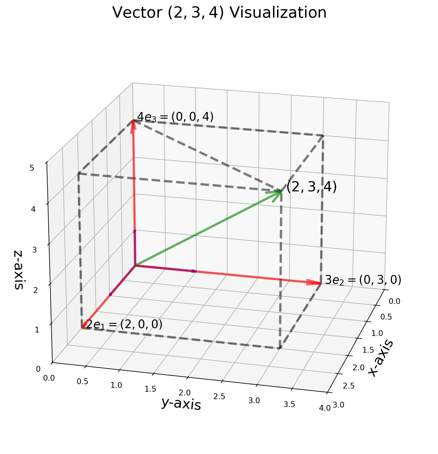

Next we show the linear combination of a non-standard basis, \((2,1,0), (0,3,1), (0,0,3)\). I also wrote another function linearComboNonStd in the linear_algebra_visulization module.

a, b, c = 2, 3, 4
vec1 = np.array([2, 1, 0])
vec2 = np.array([0, 3, 1])
vec3 = np.array([1, 2, 3])
linear_algebra_visulization.linearComboNonStd(2, 3, 4, vec1, vec2, vec3)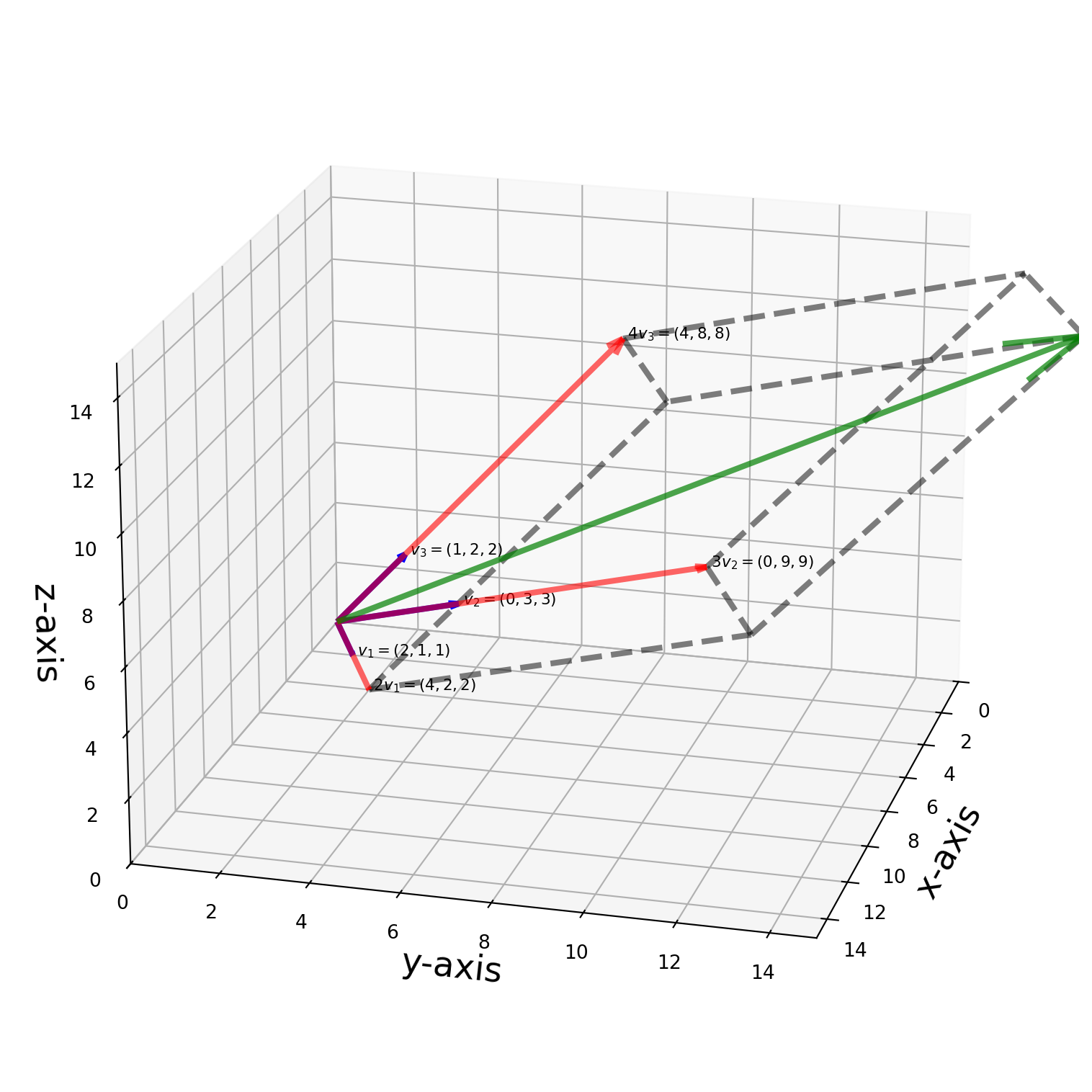

Dimension

If \(B = \{v_1, v_2, ..., v_n\}\) is the basis for \(V\), then the number of vectors in \(B\) is the dimension of \(V\), denoted as \(\text{dim}(V)\).

Theorem 1

Let \(B\) be the basis of \(V\), \(B\) has \(n\) vectors, and \(T\) is a set of vectors in \(V\), if \(T\) has \(p\) vectors that \(p>n\), then \(T\) must be linearly dependent.

Theorem 2

If \(B\) and \(T\) both are bases of \(V\) then \(B\) and \(T\) must have the same number of vectors which is the \(\text{dim}(V)\).

Theorem 3

\(\text{dim}(V) = n\) and \(S\) is a set of vectors from \(V\) with \(n\) linearly independent vectors, then \(\text{span}(S)=V\).

Theorem 4

Let \(v_1, v_2, ...,v_n\) be a set of vectors in the vector space \(V\) and let \(W = \text{span}\{v_1,v_2,...,v_n\}\). If \(v_n\) is a linear combination of \(v_1, v_2,...v_{n-1}\), then \(W = \text{span}\{v_1,v_2,...,v_{n-1}\}\)

These theorems are self-explanatory, no need to memorize, the best way to understand them is visualize them in your mind with \(\mathbb{R}^3\).

Column Space

Columns space of a matrix is denoted as \(\text{Col}A\), which is the space spanned by all columns of a matrix.

Important Fact

Row operations will not change the dependence of the columns of a matrix.

Let’s say we have a matrix \(A\)

A = sy.Matrix([[1, -2, -1, 3, 0], [-2, 4, 5, -5, 3], [3, -6, -6, 8, 2]])
A

\(\displaystyle \left[\begin{matrix}1 & -2 & -1 & 3 & 0\\-2 & 4 & 5 & -5 & 3\\3 & -6 & -6 & 8 & 2\end{matrix}\right]\)

Perform rref operations, and dependence of \(\text{Col}A\) reserved.

A.rref()

\(\displaystyle \left( \left[\begin{matrix}1 & -2 & 0 & \frac{10}{3} & 0\\0 & 0 & 1 & \frac{1}{3} & 0\\0 & 0 & 0 & 0 & 1\end{matrix}\right], \ \left( 0, \ 2, \ 4\right)\right)\)

The \(2nd\) and the \(4th\) column are the linear combination of other vectors, it is safe remove them without tampering the column space. Therefore the \(\text{Col}A\) is

ColA = sy.Matrix([[1, -1, 0], [-2, 5, 3], [3, -6, 2]])
ColA

\(\displaystyle \left[\begin{matrix}1 & -1 & 0\\-2 & 5 & 3\\3 & -6 & 2\end{matrix}\right]\)

Column Spaces Aren’t the Same

Did you notice there was a catch when we say the dependency of \(\text{Col}A\) was not affect by row operations, however we did not say the column spaces are the same as before and after the row operations.

Actually, they can never be the same.

Consider the matrix \(A\):

A = sy.Matrix([[3, -1, -1], [2, 4, 4], [-1, 1, 1]])
A

\(\displaystyle \left[\begin{matrix}3 & -1 & -1\\2 & 4 & 4\\-1 & 1 & 1\end{matrix}\right]\)

If we perform rref, \(A\) is turned into \(B\). Apparently the column space of them are different.

B = A.rref()
B

\(\displaystyle \left( \left[\begin{matrix}1 & 0 & 0\\0 & 1 & 1\\0 & 0 & 0\end{matrix}\right], \ \left( 0, \ 1\right)\right)\)

Now list the basis of their column spaces: are \(\text{Col}A\) and \(\text{Col}B\) the same?

\[ \text{col}(A) = \text{span}\left\{\begin{pmatrix} 3 \\ 2 \\ -1 \end{pmatrix}, \ \begin{pmatrix} -1 \\ 4 \\ 1 \end{pmatrix}\right\} \]

\[ \text{col}(B) = \text{span}\left\{\begin{pmatrix} 1 \\ 0 \\ 0 \end{pmatrix}, \ \begin{pmatrix} 0 \\ 1 \\ 0 \end{pmatrix}\right\} \]

It’s easy to visualize them, they are two intersecting planes, which means it’s different column space.

fig = plt.figure(figsize=(10, 10))
ax = fig.add_subplot(projection="3d")

s = np.linspace(-2, 2, 20)
t = np.linspace(-2, 2, 20)
S, T = np.meshgrid(s, t)

X = 3 * S - T
Y = 2 * S + 4 * T
Z = -S + T
ax.plot_wireframe(X, Y, Z, linewidth=0.5, color="r")

s = np.linspace(-10, 10, 20)
t = np.linspace(-10, 10, 20)
S, T = np.meshgrid(s, t)
X = S
Y = T
Z = np.zeros(S.shape)
ax.plot_wireframe(X, Y, Z, linewidth=0.5, color="k")
ax.view_init(elev=14, azim=58)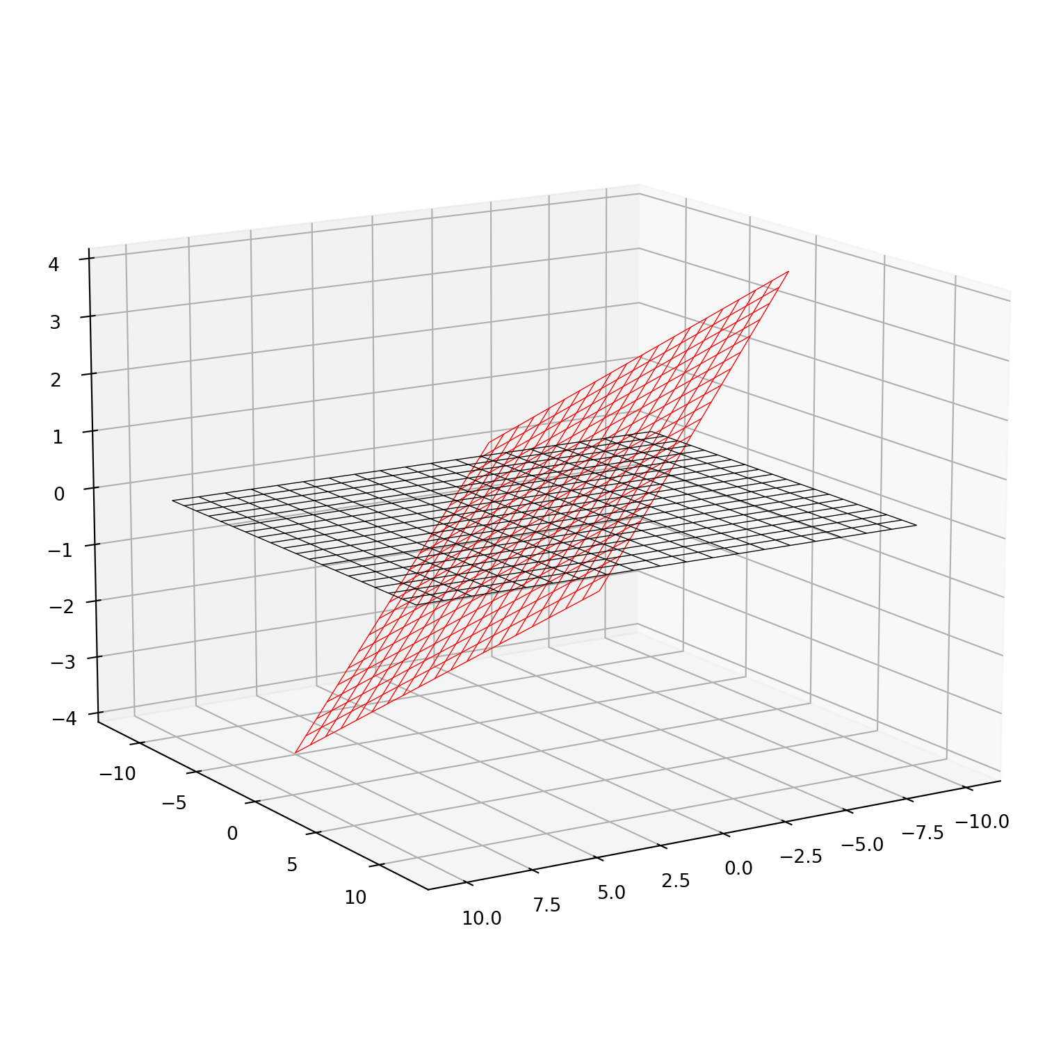

Method for Finding Basis of \(\mathbb{R}^n\)

Consider matrix \(A_{4\times 2}\), find a basis for \(\mathbb{R}^4\).

Note that we only have two column vectors, not possible to span \(\mathbb{R}^4\). The common method is to use another two standard basis vectors joined with \(A\) to form the basis of \(\mathbb{R}^4\).

A = sy.randMatrix(4, 2)
A

\(\displaystyle \left[\begin{matrix}99 & 3\\36 & 43\\73 & 81\\14 & 42\end{matrix}\right]\)

I = sy.eye(4)
I

\(\displaystyle \left[\begin{matrix}1 & 0 & 0 & 0\\0 & 1 & 0 & 0\\0 & 0 & 1 & 0\\0 & 0 & 0 & 1\end{matrix}\right]\)

Concatenate the matrix horizontally.

Aug = A.row_join(I)
Aug  # concatenate

\(\displaystyle \left[\begin{matrix}99 & 3 & 1 & 0 & 0 & 0\\36 & 43 & 0 & 1 & 0 & 0\\73 & 81 & 0 & 0 & 1 & 0\\14 & 42 & 0 & 0 & 0 & 1\end{matrix}\right]\)

Aug.rref()

\(\displaystyle \left( \left[\begin{matrix}1 & 0 & 0 & 0 & \frac{1}{46} & - \frac{27}{644}\\0 & 1 & 0 & 0 & - \frac{1}{138} & \frac{73}{1932}\\0 & 0 & 1 & 0 & - \frac{49}{23} & \frac{650}{161}\\0 & 0 & 0 & 1 & - \frac{65}{138} & - \frac{223}{1932}\end{matrix}\right], \ \left( 0, \ 1, \ 2, \ 3\right)\right)\)

Therefore the first 4 columns of augmented matrix is a basis.

Aug[:, 0:4]

\(\displaystyle \left[\begin{matrix}99 & 3 & 1 & 0\\36 & 43 & 0 & 1\\73 & 81 & 0 & 0\\14 & 42 & 0 & 0\end{matrix}\right]\)

Change of Basis

Change of basis is for changing the coordinate system,e.g. from Cartesian to other system.

Coordinate Vector

We have a basis \(B=\{b_1, b_2\}\), and \(B\)’s coordinate vector is denoted as \(\big[v\big]_B\). If

\[ b_1 = \left[\begin{matrix}1\\1 \end{matrix}\right]\\ b_2 = \left[\begin{matrix}-2\\1 \end{matrix}\right]\\ \big[v\big]_B = \left[\begin{matrix}2\\3 \end{matrix}\right] \]

Then compute \(v\) by using the basis and its coordinate vectors. We want to convert the \(\big[v\big]_B\) into a pair of Cartesian coordinates.

P = sy.Matrix([[1, -2], [1, 1]])
P

\(\displaystyle \left[\begin{matrix}1 & -2\\1 & 1\end{matrix}\right]\)

v_B = sy.Matrix([[2], [3]])
v_B

\(\displaystyle \left[\begin{matrix}2\\3\end{matrix}\right]\)

P * v_B

\(\displaystyle \left[\begin{matrix}-4\\5\end{matrix}\right]\)

Now we have successfully converted \(\big[v\big]_B\) into Cartesian

On the other way around, what if we know \(v\) i.e. the Cartesian coordinates, and we want to find out \(\big[v\big]_B\), for instance

\[ v = \left[\begin{matrix}-1\\-4 \end{matrix}\right] \]

Then we can formulate the question as:

\[ \left[\begin{matrix}1 & -2\\1 & 1\end{matrix}\right] \left[\begin{matrix}b_1\\b_2 \end{matrix}\right]= \left[\begin{matrix}-1\\-4 \end{matrix}\right] \]

Just solve the linear system

Aug = sy.Matrix([[1, -2, -1], [1, 1, -4]])
Aug.rref()

\(\displaystyle \left( \left[\begin{matrix}1 & 0 & -3\\0 & 1 & -1\end{matrix}\right], \ \left( 0, \ 1\right)\right)\)

We get \(\big[v\big]_B = (-3, -1)^T\).

Change of Basis

Most probably we would like to change coordinates from \(\big[v\big]_B\) to \(\big[v\big]_C\), which both aren’t Cartesian coordinates.

Say we have two bases \(B=\{b_1,\ b_2\}\), \(C=\{c_1,\ c_2\}\) in \(\mathbb{R}^2\).

\[ b_1= \left[\begin{matrix}2\\1 \end{matrix}\right],\quad b_2 = \left[\begin{matrix}-1\\1 \end{matrix}\right]\\ c_1= \left[\begin{matrix}1\\1 \end{matrix}\right],\quad c_2 = \left[\begin{matrix}-3\\1 \end{matrix}\right]\\ \]

We would like to change \(\big[v\big]_B\) to \(\big[v\big]_C\). Formally this is reformulated as finding transition matrix \(P_{C\leftarrow B}\).

First we find coordinate vectors for \(b_1\) and \(b_2\) in \(C: b_1 = xc_1+yc_2\), \(b_2 = xc_1+yc_2\).

\[ \left[\begin{matrix}2\\1 \end{matrix}\right] = x\left[\begin{matrix}1\\1 \end{matrix}\right]+y\left[\begin{matrix}-3\\1 \end{matrix}\right]= \left[\begin{matrix}1 & -3\\1 &1 \end{matrix}\right]\left[\begin{matrix}x \\y \end{matrix}\right]\\ \left[\begin{matrix}-1\\1 \end{matrix}\right] = x\left[\begin{matrix}1\\1 \end{matrix}\right]+y\left[\begin{matrix}-3\\1 \end{matrix}\right]=\left[\begin{matrix}1 & -3\\1 &1 \end{matrix}\right]\left[\begin{matrix}x \\y \end{matrix}\right]\\ \]

Extract augmented matrix for both system:

\[ \left[\begin{matrix}1 & -3 & 2\\1 &1 &1 \end{matrix}\right]\\ \left[\begin{matrix}1 & -3 & -1\\1 &1 &1 \end{matrix}\right] \]

They can be combined into one augmented matrix \([C|B]\)

\[ \left[\begin{matrix}1 & -3 & 2 & -1\\1 &1 &1 &1 \end{matrix}\right] \]

Aug = sy.Matrix([[1, -3, 2, -1], [1, 1, 1, 1]])
Aug.rref()

\(\displaystyle \left( \left[\begin{matrix}1 & 0 & \frac{5}{4} & \frac{1}{2}\\0 & 1 & - \frac{1}{4} & \frac{1}{2}\end{matrix}\right], \ \left( 0, \ 1\right)\right)\)

The last two columns of rref augmented matrix is the \(P_{C\leftarrow B}\).

In general, we can find transition matrix by using

\[[\ C\ |\ B\ ]\longrightarrow [\ I\ |\ P_{C\leftarrow B}\ ]\]

An Example

Let

\[ B=\left\{\left[\begin{array}{l} 1 \\ 1 \\ 0 \end{array}\right],\left[\begin{array}{l} 0 \\ 1 \\ 1 \end{array}\right],\left[\begin{array}{l} 0 \\ 1 \\ 0 \end{array}\right]\right\} \quad \text { and } \quad C=\left\{\left[\begin{array}{l} 1 \\ 1 \\ 2 \end{array}\right],\left[\begin{array}{l} 2 \\ 1 \\ 1 \end{array}\right],\left[\begin{array}{l} 1 \\ 0 \\ 1 \end{array}\right]\right\} \]

be two bases for \(\mathbb{R}^3\), find the \(P_{C\leftarrow B}\) and given \(\big[v\big]_B = (1,-1,2)\), find \(\big[v\big]_C\).

Construct augmented matrix:

v_B = sy.Matrix([1, -1, 2])
B = sy.Matrix([[1, 0, 0], [1, 1, 1], [0, 1, 0]])
C = sy.Matrix([[1, 2, 1], [1, 1, 0], [2, 1, 1]])
Aug = C.row_join(B)
Aug  # concatenate

\(\displaystyle \left[\begin{matrix}1 & 2 & 1 & 1 & 0 & 0\\1 & 1 & 0 & 1 & 1 & 1\\2 & 1 & 1 & 0 & 1 & 0\end{matrix}\right]\)

The RHS block of rref is \(P_{C\leftarrow B}\) as we have shown above.

Aug_rref = Aug.rref()
Aug_rref

\(\displaystyle \left( \left[\begin{matrix}1 & 0 & 0 & 0 & 1 & \frac{1}{2}\\0 & 1 & 0 & 1 & 0 & \frac{1}{2}\\0 & 0 & 1 & -1 & -1 & - \frac{3}{2}\end{matrix}\right], \ \left( 0, \ 1, \ 2\right)\right)\)

v_C = Aug_rref[0][:, 3:6] * v_B
v_C

\(\displaystyle \left[\begin{matrix}0\\2\\-3\end{matrix}\right]\)

The \(\big[v\big]_C\) is \((0, 2, -3)\).