import matplotlib.pyplot as plt
import numpy as np
import sympy as sy

sy.init_printing()
If all \(c\)’s are zero, a set of vectors \(\{v_1, v_2,...,v_p\}\) is said to be linearly independent, if the equation
\[c_{1} {v}_{1}+c_{2} {v}_{2}+\cdots+c_{p} {v}_{p}=\mathbf{0}\]
holds.
If any of \(c_i\neq 0\), the set of vectors is linearly dependent.
Example 1
Determine if \({v}_1, {v}_2, {v}_3\) are linearly independent. \[ {v}_{1}=\left[\begin{array}{l} 1 \\ 2 \\ 3 \end{array}\right]^T, {v}_{2}=\left[\begin{array}{l} 4 \\ 5 \\ 6 \end{array}\right]^T, \text { and } {v}_{3}=\left[\begin{array}{l} 2 \\ 1 \\ 0 \end{array}\right]^T \]
The common way of testing linear combination is to construct augmented matrix and calculate the reduced form, for example
A = sy.Matrix([[1, 4, 2, 0], [2, 5, 1, 0], [3, 6, 0, 0]])
A.rref()
\(\displaystyle \left( \left[\begin{matrix}1 & 0 & -2 & 0\\0 & 1 & 1 & 0\\0 & 0 & 0 & 0\end{matrix}\right], \ \left( 0, \ 1\right)\right)\)
The solution tells that \(x_3\) is a free variable, so naturally it could be nonzero because \(x_3\cdot 0 =0\), therefore the set is linearly dependent.
Example 2
Consider a matrix \(A\),determine if columns of \(A\) are linearly independent.
\[ A=\left[\begin{array}{rrr} 0 & 1 & 4 \\ 1 & 2 & -1 \\ 5 & 8 & 0 \end{array}\right] \]
Solve the system via augmented matrix.
A = sy.Matrix([[0, 1, 4, 0], [1, 2, -1, 0], [5, 8, 0, 0]])
A.rref()
\(\displaystyle \left( \left[\begin{matrix}1 & 0 & 0 & 0\\0 & 1 & 0 & 0\\0 & 0 & 1 & 0\end{matrix}\right], \ \left( 0, \ 1, \ 2\right)\right)\)
\(Ax=0\) has only trivial solution, i.e. \((c_1, c_2, c_3)^T = (0, 0, 0)\), so the columns of \(A\) are linearly independent.
Linear independence is closly connected with linear combination, in next section we visualize the linear independence.
Visualization of Linear Independence
This is a visual example in \(\mathbb{R}^2\), showing \((3, 2)^T\), \((-9, -6)^T\), \((6, 4)^T\) are linearly dependent.
fig, ax = plt.subplots(figsize=(8, 8))
#######################Arrows#######################
arrows = np.array([[[0, 0, 3, 2]], [[0, 0, -9, -6]], [[0, 0, 6, 4]]])
colors = ["r", "b", "g"]
for i in range(arrows.shape[0]):
    X, Y, U, V = zip(*arrows[i, :, :])
    ax.arrow(
        X[0],
        Y[0],
        U[0],
        V[0],
        color=colors[i],
        width=0.18,
        length_includes_head=True,
        head_width=0.3,  # default: 3*width
        head_length=0.6,
        overhang=0.4,
        zorder=-i,
    )

ax.scatter(0, 0, ec="red", fc="black", zorder=5)
ax.text(6, 4, "$(6, 4)$")
ax.text(-9, -6.5, "$(-9, -6)$")
ax.text(3, 2, "$(3, 2)$")

ax.grid(True)
ax.set_title("Linear Dependence Visualization")
ax.axis([-10, 10, -10, 10])
ax.set_xlabel("x-axis", size=18)
ax.set_ylabel("y-axis", size=18)
plt.show()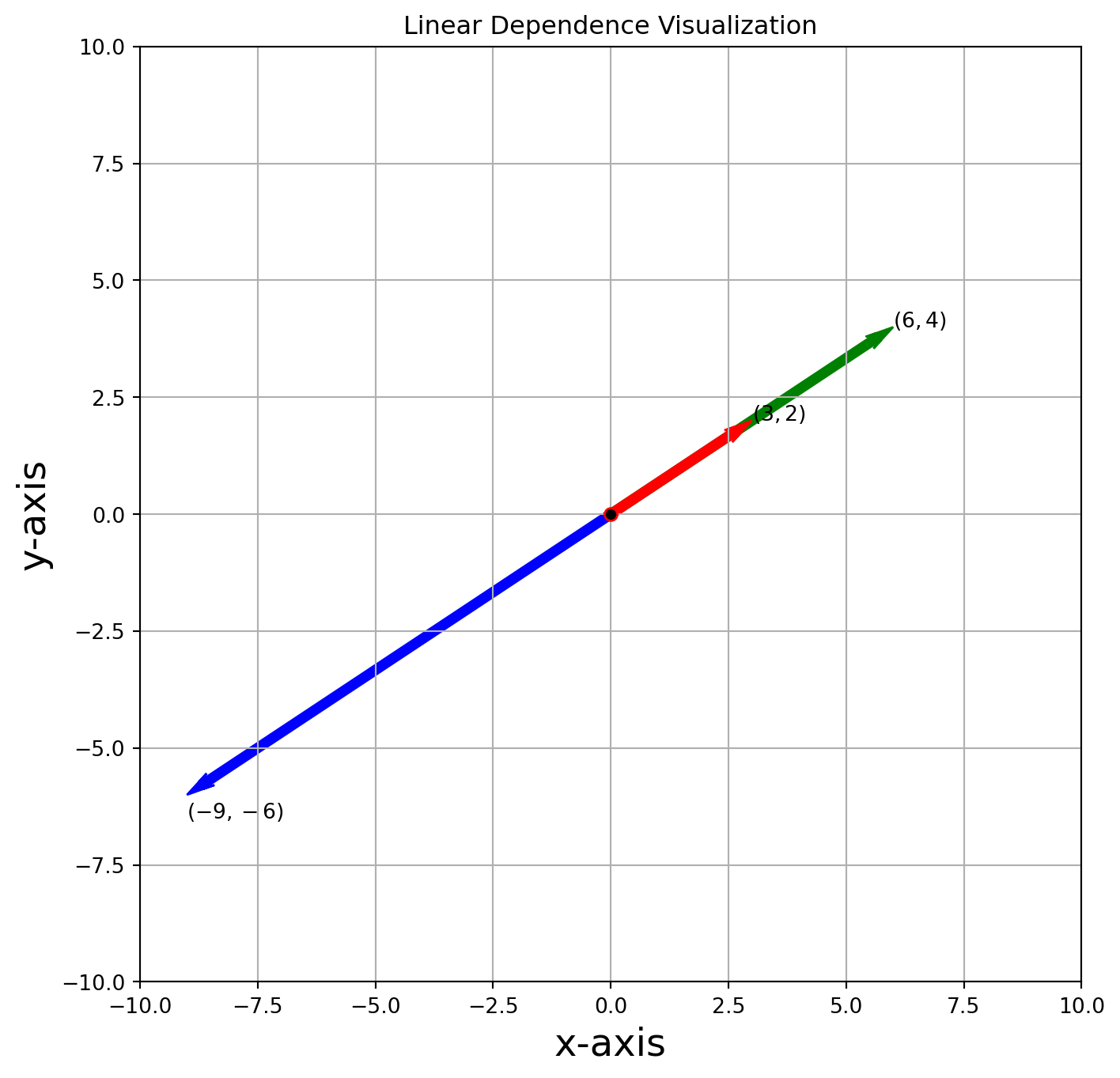
Simply put, if one vector is the scalar multiple of the other vector, e.g. \(3u = v\), these two vectors are linearly dependent.
Next, we visualize linear independence in \(\mathbb{R}^3\) with vectors \((1,-2,1)^T\), \((2,1,2)^T\), \((-1,2,3)^T\).
The standard procedure is to write down the span of first two vectors, which is a plane. Then we examine whether the third vector is in the plane. If not, this set of vectors is linearly independent.
\[ \left[ \begin{matrix} x\\ y\\ z \end{matrix} \right]= s\left[ \begin{matrix} 1\\ -2\\ 1 \end{matrix} \right]+ t\left[ \begin{matrix} 2\\ 1\\ 2 \end{matrix} \right]= \left[ \begin{matrix} s+2t\\ -2s+t\\ s+2t \end{matrix} \right] \]
# %matplotlib notebook, use this only when you are in Jupyter Notebook, it doesn't work in Jupyterlab
fig = plt.figure(figsize=(10, 10))
ax = fig.add_subplot(projection="3d")

s = np.linspace(-1, 1, 10)
t = np.linspace(-1, 1, 10)
S, T = np.meshgrid(s, t)

X = S + 2 * T
Y = -2 * S + T
Z = S + 2 * T
ax.plot_wireframe(X, Y, Z, linewidth=1.5, color="k", alpha=0.6)

vec = np.array([[[0, 0, 0, 1, -2, 1]], [[0, 0, 0, 2, 1, 2]], [[0, 0, 0, -1, 2, 3]]])
colors = ["r", "b", "g"]
for i in range(vec.shape[0]):
    X, Y, Z, U, V, W = zip(*vec[i, :, :])
    ax.quiver(
        X,
        Y,
        Z,
        U,
        V,
        W,
        length=1,
        normalize=False,
        color=colors[i],
        arrow_length_ratio=0.08,
        pivot="tail",
        linestyles="solid",
        linewidths=3,
        alpha=0.6,
    )

ax.set_title("Linear Independence Visualization")

ax.set_xlabel("x-axis", size=18)
ax.set_ylabel("y-axis", size=18)
ax.set_zlabel("z-axis", size=18)

ax.view_init(elev=50.0, azim=0)
plt.show()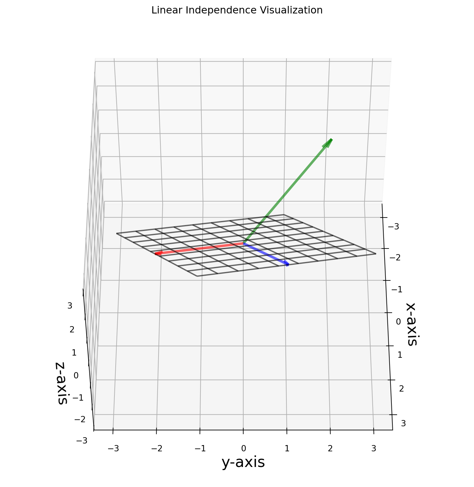
Pan around the image (either by setting ax.view_init or using JupyterLab widget), we can see that the green vector is not in the plane spanned by red and blue vector, thus they are linearly independent.
A Sidenote About Linear Independence
Let \(S = \{{v}_1,{v}_2,{v}_3, ..., {v}_n\}\) be a set of vectors in \(\mathbb{R}^m\), if \(n>m\), then \(S\) is always linearly dependent. Simple example is \(4\) vectors in \(\mathbb{R}^3\), even if \(3\) of them are linearly independent, the \(4\)-th one can never be independent of them.
Also if \(S = \{{v}_1,{v}_2,{v}_3, ..., {v}_n\}\) contains a zero vector, then the set is always linearly dependent.