The Singular Values

import numpy as np
import scipy as sp
import sympy as sy
import matplotlib.pyplot as plt

plt.style.use("ggplot")

np.set_printoptions(precision=3)
np.set_printoptions(suppress=True)

We have discussed what Spectral Decomposition which can decompose any symmetric matrices unconditionally into three special matrices.However only square matrices have eigenvalues and vectors, however we want to extend a similar concept for any \(m \times n\) matrices.

If \(A\) is an \(m \times n\) matrix, then \(A^TA\) and \(AA^T\) are both symmetric and orthogonally diagonalizable.

A = np.array([[4, -3], [-3, 2], [2, -1], [1, 0]])
A

array([[ 4, -3],
       [-3,  2],
       [ 2, -1],
       [ 1,  0]])

Compute eigenvalues and eigenvectors of \(A^TA\).

ATA = A.T @ A
ATA

array([[ 30, -20],
       [-20,  14]])

D1, P1 = np.linalg.eig(ATA)

Check if \(P\) is an orthonormal matrix.

P1 @ P1.T

array([[1., 0.],
       [0., 1.]])

D1

array([43.541,  0.459])

The square roots of eigenvalues of \(A^TA\) are called singular values of \(A\), denoted by \(\sigma_1, ..., \sigma_n\) in decreasing order.

We can also show that singular values of \(A\) are the lengths of vectors \(A\mathbf{v}_1,..., A\mathbf{v}_n\), where \(\mathbf{v}_i\) is the eigenvalue of \(A^TA\).

The length of \(A\mathbf{v}_i\) is \(\|A\mathbf{v}_i\|\)

\[ \|A\mathbf{v}_i\| = \sqrt{(A\mathbf{v}_i)^TA\mathbf{v}_i} = \sqrt{\mathbf{v}_i^TA^T A\mathbf{v}_i}=\sqrt{\mathbf{v}_i^T(\lambda_i\mathbf{v}_i)} = \sqrt{\lambda_i}=\sigma_1 \]

where \(\sqrt{\mathbf{v}_i^T\mathbf{v}_i} = 1\) and \(\lambda_i\)’s are eigenvalues of \(A^TA\).

# Singular Value Decomposition

Singular Value Decomposition (SVD) is probably the most important decomposition technique in the history of linear algebra, it combines all the theory we discussed, then culminate at this point.

\(A\) is a \(m\times n\) matrix. However \(AA^T\) and \(A^TA\) are symmetric matrices,then both are orthogonally diagonalizable.

\[ AA^T = U\Sigma\Sigma^T U^T=(U\Sigma V^T)(V\Sigma U^T)\\ A^TA = V\Sigma^T \Sigma V^T = (V\Sigma^T U^T)(U \Sigma V^T) \]

where \(\Sigma\Sigma^T\) is a diagonal matrix with all eigenvalues of \(AA^T\) and \(\Sigma^T \Sigma\) is a diagonal matrix with all eigenvalues of \(VV^T\).

Because both \(AA^T\) and \(A^TA\) are symmetric, then \(UU^T= U^TU=I_{m\times m}\) and \(VV^T= V^TV=I_{n\times n}\).

We have implicitly shown the singular value decompositions above, one of the most important concept in linear algebra.

\[ \Large SVD:\quad A_{m\times n} = U_{m\times m}\Sigma_{m \times n} V^T_{n \times n} \]

The SVD theory guarantees that any matrix \(A\), no matter its ranks or shapes, can be unconditionally decomposed into three special matrices.

So next question: what is \(\Sigma\)?

It is an \(m\times n\) main diagonal matrix, with all singular values on the main diagonal. Rewrite

\[ A^TA = V\Sigma^T \Sigma V^T = V\Sigma^2 V^T \]

Post-multiply both sides by \(V\)

\[ A^TAV = V\Sigma^2 \]

This is the matrix version of \(A\mathbf{v}_i = \lambda_i \mathbf{v}_i\), but here the matrix of interest is \(A^TA\) rather than \(A\). Similarly it can be written with singular values

\[ A^TA\mathbf{v}_i = \sigma_i^2\mathbf{v}_i \]

Because \(U\) and \(V\) are not unique, we tend to standardize the solution by arranging \(\sigma_1 \geq \sigma_2 \geq \sigma_3\geq ... \geq\sigma_r\).

Why we only arrange \(r\) singular values? Because it is the rank of \(A\), so is the rank of \(A^TA\). Explicitly \(\Sigma\) looks like

\[\Sigma =\left[\begin{array}{cccccc} \sqrt{\lambda_{1}} & & & & &\\ & \sqrt{\lambda_{2}} & & & &\\ & & \ddots & & &\\ & & & \sqrt{\lambda}_{\mathrm{r}} & &\\ & & & & \ddots &\\ & & & & & 0 \end{array}\right] =\left[\begin{array}{cccccc} \sigma_1 & & & & &\\ & \sigma_2 & & & &\\ & & \ddots & & &\\ & & & \sigma_r & &\\ & & & & \ddots &\\ & & & & & 0 \end{array}\right] \]

We can do the same for \(AA^T\) and get

\[ AA^TU = U \Sigma^2 \]

or

\[ AA^T\mathbf{u}_i = \sigma_i^2\mathbf{u}_i \]

We have shown why \(A_{m\times n} = U_{m\times m}\Sigma_{m \times n} V^T_{n \times n}\) holds.

To perfomr a SVD on \(A\), we just need two equations and this is also a mannual procedure to decompose any matrix.

\[ A^TA = V\Sigma^T \Sigma V^T\\ AV = U\Sigma \]

Here’s an example, let’s say we have we have a data set \(A\)

A = np.random.rand(10, 2)

Give it a \(\text{SVD}\) decomposition

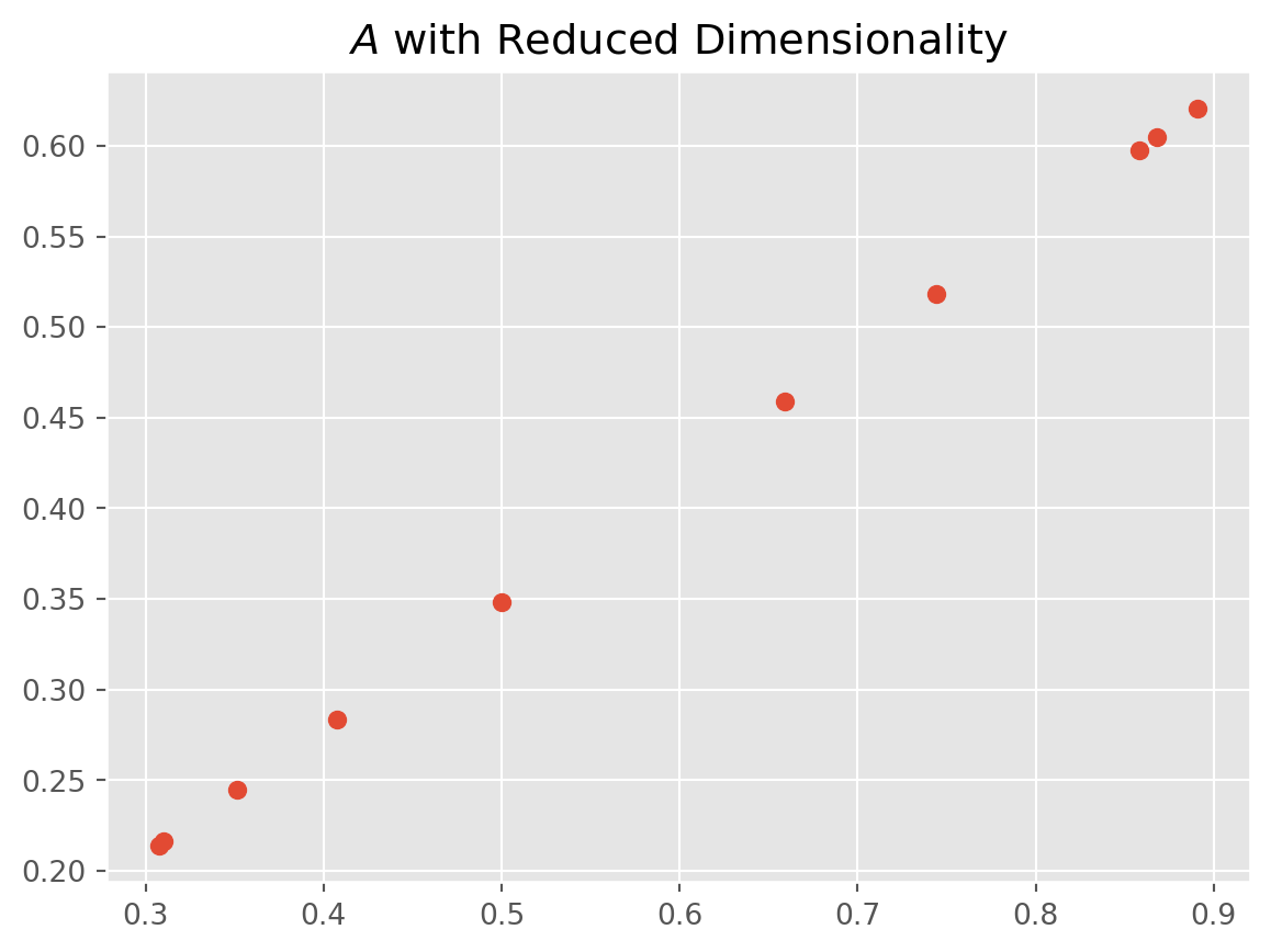
U, S, VT = np.linalg.svd(A, full_matrices=False)

Let’s say we want to reduce \(A_{10\times 3}\) in to \(A_{10\times 2}\).

# Keep only the first dimension
A_reduced = np.dot(U[:, :1], np.dot(np.diag(S[:1]), VT[:1, :]))

# Plot original data
plt.scatter(A[:, 0], A[:, 1])
plt.title("Original $A$")
plt.show()

# Plot reduced data
plt.scatter(A_reduced[:, 0], A_reduced[:, 1])
plt.title("$A$ with Reduced Dimensionality")
plt.show()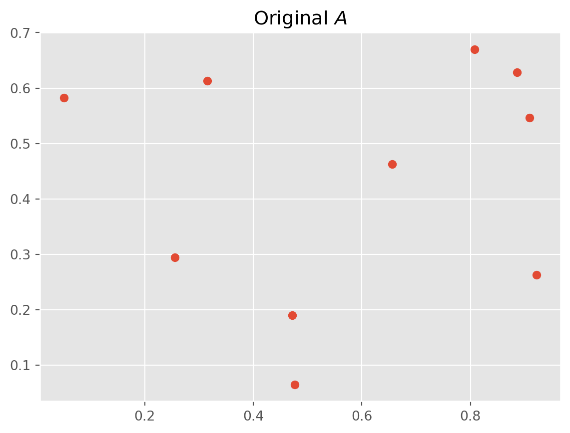

import numpy as np
import matplotlib.pyplot as plt

# Generate some random data
np.random.seed(0)
data = np.random.randn(200, 2)

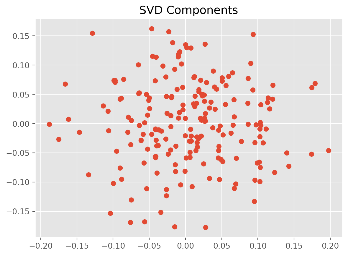
# Perform SVD on the data
U, s, VT = np.linalg.svd(data)

# Perform PCA on the data
mean = np.mean(data, axis=0)
data_pca = data - mean
cov = np.cov(data_pca.T)
eigenvalues, eigenvectors = np.linalg.eig(cov)

# Plot the data
plt.scatter(data[:, 0], data[:, 1])
plt.title("Original Data")
plt.show()

# Plot the SVD components
plt.scatter(U[:, 0], U[:, 1])
plt.title("SVD Components")
plt.show()

# Plot the PCA components
plt.scatter(eigenvectors[:, 0], eigenvectors[:, 1])
plt.title("PCA Components")
plt.show()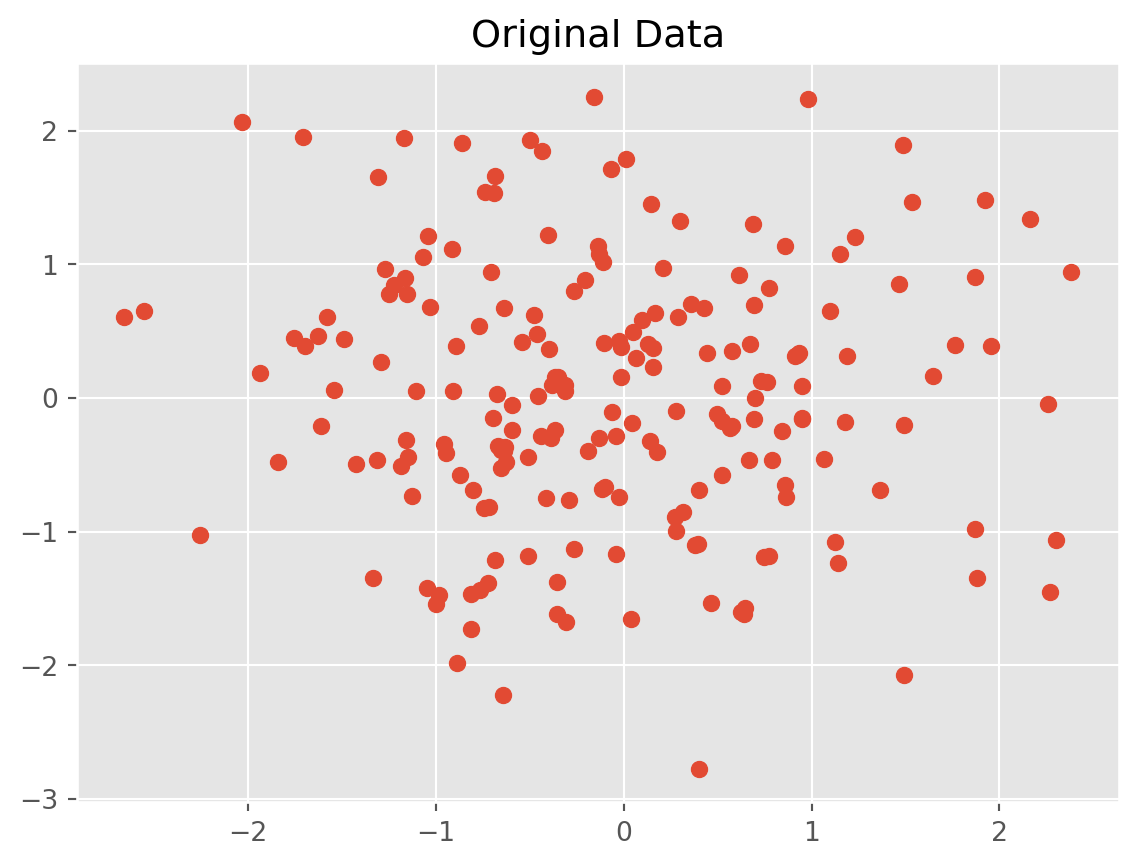

Reformulate SVD

Rewrite \(SVD\)

\[ AV = U\Sigma \]

vector version is

\[ A\mathbf{v}_i = \sigma_i \mathbf{u}_i \]

There two implications from the equation above: \((a)\) \(A\) can be decomposed into

\[ A = \sum_{i}^r\sigma_i\mathbf{u}_i \mathbf{v}_i^T \]

\((b)\) We can compute \(\mathbf{u}_i\) by using

\[\mathbf{u}_i = \frac{A\mathbf{v}_i}{\sigma_i}\]