import matplotlib.pyplot as plt
import numpy as np
import scipy as sp
import sympy as sy
import plotly.graph_objects as go

sy.init_printing()

Consider two vectors

\[ \mathbf{u}=\left[\begin{array}{l} u_{1} \\ u_{2} \\ \vdots \\ u_{n} \end{array}\right] \quad \text { and } \bf{v}=\left[\begin{array}{l} v_{1} \\ v_{2} \\ \vdots \\ v_{n} \end{array}\right] \]

The dot product of $\mathbf{u}$ and $\mathbf{v}$, i.e. $\mathbf{u}\cdot\mathbf{v}$ is defined as

\[ \left[\begin{array}{llll} u_{1} & u_{2} & \cdots & u_{n} \end{array}\right]\left[\begin{array}{c} v_{1} \\ v_{2} \\ \vdots \\ v_{n} \end{array}\right]=u_{1} v_{1}+u_{2} v_{2}+\cdots+u_{n} v_{n} \]

We can generate two random vectors, then let’s compare operations in NumPy.

u = np.round(100 * np.random.randn(10))
v = np.round(100 * np.random.randn(10))

u * v  # this is element-wise multiplication

array([ -1696.,   1794., -10824.,  -7626.,    246.,  -2256.,  -6431.,
         2496.,   1054.,   2730.])

u @ v  # matrix multiplication, which is a dot product in this case

$\displaystyle -20513.0$

np.inner(u, v)  # inner product here is the same as matrix multiplication

$\displaystyle -20513.0$

The Norm of a Vector

The norm is the length of a vector, defined by

\[ \|\mathbf{v}\| = \sqrt{\mathbf{v} \cdot \mathbf{v}} = \sqrt{v_{1}^{2} + v_{2}^{2} + \cdots + v_{n}^{2}}, \quad \text{and} \quad \|\mathbf{v}\|^{2} = \mathbf{v} \cdot \mathbf{v} \]

The NumPy built-in function np.linalg.norm() is used for computing norms. By default, it computes the length of vectors from the origin.

a = [2, 6]
np.linalg.norm(a)

$\displaystyle 6.32455532033676$

Verify the results.

np.sqrt(2**2 + 6**2)

$\displaystyle 6.32455532033676$

This function can also compute a group of vectors’ length, for instance $(2, 6)^T$, $(8, 2)^T$, $(9, 1)^T$

A = np.array([[2, 8, 9], [6, 2, 1]])
np.linalg.norm(A, axis=0)

array([6.32455532, 8.24621125, 9.05538514])

Distance in $\mathbb{R}^n$

For $\mathbf{u}$ and $\mathbf{v}$ in $\mathbb{R}^{n}$, the distance between $\mathbf{u}$ and $\mathbf{v},$ written as dist $(\mathbf{u}, \mathbf{v}),$ is the length of the vector $\mathbf{u}-\mathbf{v} .$ That is,

\[ \operatorname{dist}(\mathbf{u}, \mathbf{v})=\|\mathbf{u}-\mathbf{v}\| \]

Suppose we have two vectors $\mathbf{u} = (2, 9)$ and $\mathbf{v} = (-3, 4)$, compute the distance and visualize the results.

u = np.array([2, 9])
v = np.array([-3, 4])
np.linalg.norm(u - v)

$\displaystyle 7.07106781186548$

fig, ax = plt.subplots(figsize=(12, 12))

# Define the vectors
vects = np.array([[2, 9], [-3, 4], [3, -4], [5, 5]])
col = ["red", "blue", "blue", "green"]
cordt = ["$(2, 9)$", "$(-3, 4)$", "$(3, -4)$", "$(5, 5)$"]

# Plot the vectors
for i in range(4):
    ax.arrow(
        0,
        0,
        vects[i, 0],
        vects[i, 1],
        color=col[i],
        width=0.08,
        length_includes_head=True,
        head_width=0.3,  # default: 3*width
        head_length=0.6,
        overhang=0.4,
    )
    ax.text(x=vects[i][0], y=vects[i][1], s=cordt[i], size=15)
ax.grid()

# Define the points for the arrows and lines
points = np.array([[2, 9], [5, 5], [3, -4], [-3, 4]])

# Plot the green vector from (-3, 4) to (2, 9)
start_point = points[3]
end_point = points[0]
direction = end_point - start_point
ax.arrow(
    start_point[0],
    start_point[1],
    direction[0],
    direction[1],
    color="green",
    width=0.08,
    length_includes_head=True,
    head_width=0.3,  # default: 3*width
    head_length=0.6,
    overhang=0.4,
)

# Plot the blue dashed lines
line1 = np.array([points[0], points[1]])
ax.plot(line1[:, 0], line1[:, 1], c="b", lw=3.5, alpha=0.5, ls="--")

line2 = np.array([points[2], points[1]])
ax.plot(line2[:, 0], line2[:, 1], c="b", lw=3.5, alpha=0.5, ls="--")

# Add the text for the distance using raw string
ax.text(-2, 6, r"$\|\|\mathbf{u}-\mathbf{v}\|\|$", size=16)

###################### Axis, Spines, Ticks ##########################
ax.axis([-10, 10.1, -10.1, 10.1])
ax.spines["left"].set_position("center")
ax.spines["right"].set_color("none")
ax.spines["bottom"].set_position("center")
ax.spines["top"].set_color("none")
ax.xaxis.set_ticks_position("bottom")
ax.yaxis.set_ticks_position("left")

ax.minorticks_on()
ax.tick_params(axis="both", direction="inout", length=12, width=2, which="major")
ax.tick_params(axis="both", direction="inout", length=10, width=1, which="minor")

plt.show()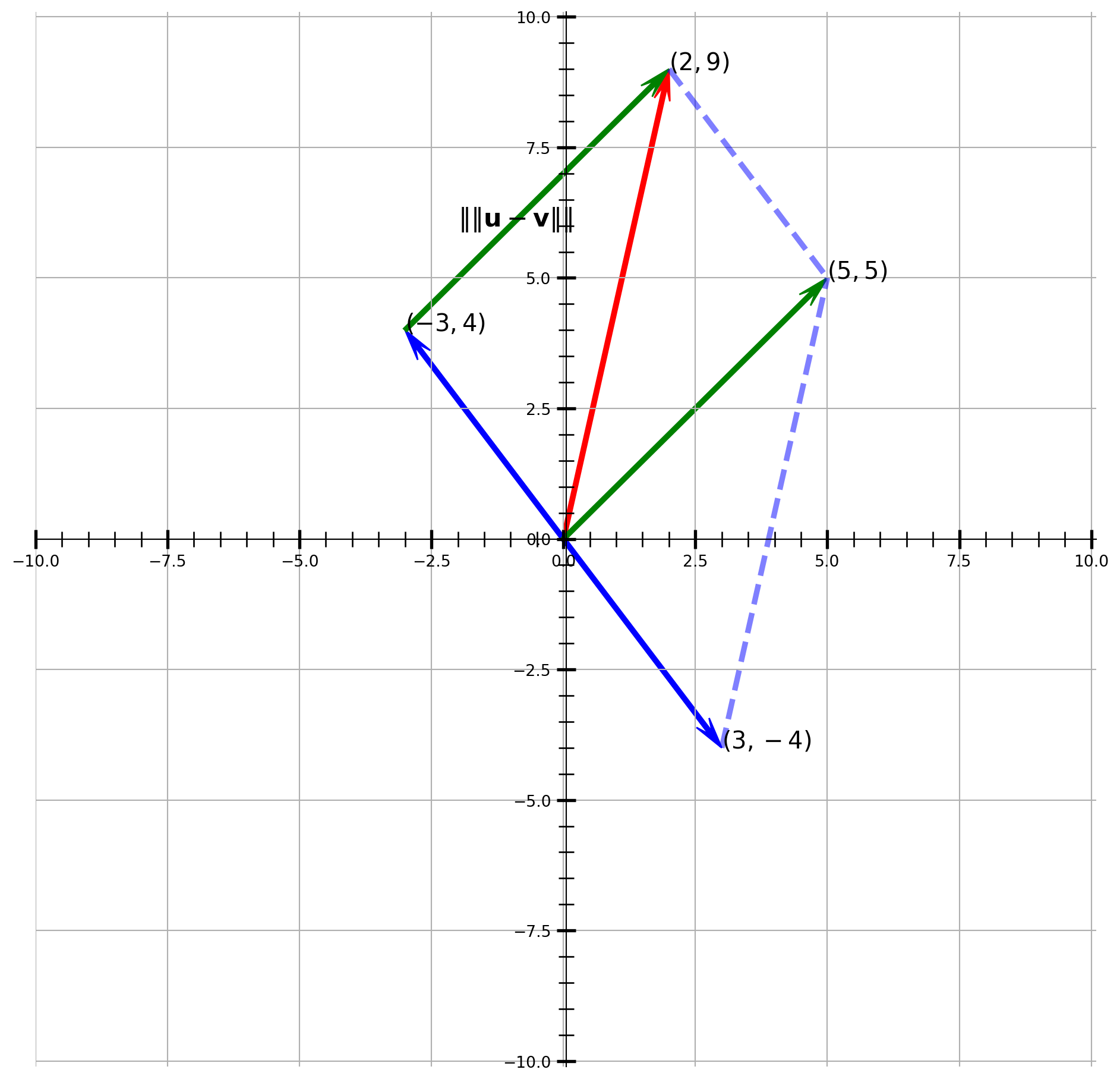

From the graph, we know that the $\|\mathbf{u}-\mathbf{v}\|$ is $\sqrt{5^2 + 5^2}$.

np.sqrt(5**2 + 5**2)

$\displaystyle 7.07106781186548$

The same results as the np.linalg.norm(u - v).

Orthogonal Vectors

We have two vectors $\mathbf{u}$ and $\mathbf{v}$, and square the distance of $\|\mathbf{u}+\mathbf{v}\|$ and $\|\mathbf{u}-\mathbf{v}\|$

\[\begin{aligned} \big[\operatorname{dist}(\mathbf{u},-\mathbf{v})\big]^{2} &=\|\mathbf{u}-(-\mathbf{v})\|^{2}=\|\mathbf{u}+\mathbf{v}\|^{2} \\ &=(\mathbf{u}+\mathbf{v}) \cdot(\mathbf{u}+\mathbf{v}) \\ &=\mathbf{u} \cdot(\mathbf{u}+\mathbf{v})+\mathbf{v} \cdot(\mathbf{u}+\mathbf{v}) \\ &=\mathbf{u} \cdot \mathbf{u}+\mathbf{u} \cdot \mathbf{v}+\mathbf{v} \cdot \mathbf{u}+\mathbf{v} \cdot \mathbf{v} \\ &=\|\mathbf{u}\|^{2}+\|\mathbf{v}\|^{2}+2 \mathbf{u} \cdot \mathbf{v} \end{aligned}\]

\[\begin{aligned} \big[\operatorname{dist}(\mathbf{u}, \mathbf{v})\big]^{2} &=\|\mathbf{u}\|^{2}+\|-\mathbf{v}\|^{2}+2 \mathbf{u} \cdot(-\mathbf{v}) \\ &=\|\mathbf{u}\|^{2}+\|\mathbf{v}\|^{2}-2 \mathbf{u} \cdot \mathbf{v} \end{aligned}\]

Suppose $\mathbf{u} = (1, 4)$ and $\mathbf{v} = (-2, 2)$, visualize the vector and distances.

fig, ax = plt.subplots(figsize=(12, 12))

vects = np.array([[1, 4], [-2, 2], [2, -2]])
colr = ["red", "blue", "blue"]
cordt = ["$(1, 4)$", "$(-2, 2)$", "$(2, -2)$"]
vec_name = [r"$\mathbf{u}$", r"$\mathbf{v}$", r"$\mathbf{-v}$"]

for i in range(3):
    ax.arrow(
        0,
        0,
        vects[i][0],
        vects[i][1],
        color=colr[i],
        width=0.08,
        length_includes_head=True,
        head_width=0.3,  # default: 3*width
        head_length=0.6,
        overhang=0.4,
    )
    ax.text(x=vects[i][0], y=vects[i][1], s=cordt[i], size=15)
    ax.text(x=vects[i][0] / 2, y=vects[i][1] / 2, s=vec_name[i], size=22)

ax.text(x=-1, y=3, s=r"$\|\|\mathbf{u}-\mathbf{v}\|\|$", size=15)
ax.text(x=1.5, y=1, s=r"$\|\|\mathbf{u}+\mathbf{v}\|\|$", size=15)

############################### Dashed Line #######################
line1 = np.array([vects[0], vects[1]])
ax.plot(line1[:, 0], line1[:, 1], c="b", lw=3.5, alpha=0.5, ls="--")

line2 = np.array([vects[0], vects[2]])
ax.plot(line2[:, 0], line2[:, 1], c="b", lw=3.5, alpha=0.5, ls="--")

###################### Axis, Spines, Ticks ##########################
ax.spines["left"].set_position("center")
ax.spines["right"].set_color("none")
ax.spines["bottom"].set_position("center")
ax.spines["top"].set_color("none")
ax.xaxis.set_ticks_position("bottom")
ax.yaxis.set_ticks_position("left")

ax.minorticks_on()
ax.tick_params(axis="both", direction="inout", length=12, width=2, which="major")
ax.tick_params(axis="both", direction="inout", length=10, width=1, which="minor")

ax.axis([-5, 5, -5, 5])
ax.grid()

plt.show()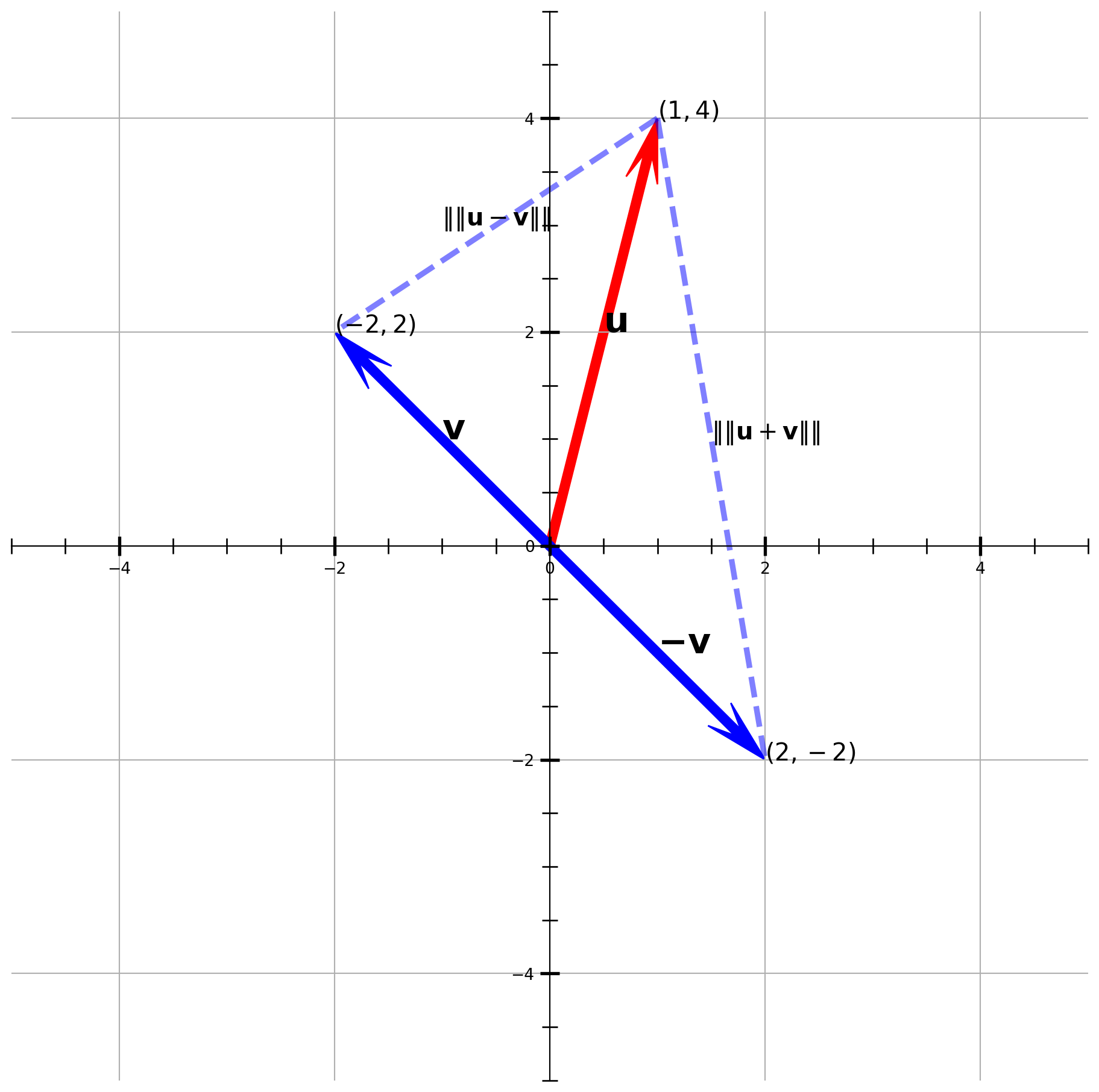

Note that if $\big[\operatorname{dist}(\mathbf{u},-\mathbf{v})\big]^{2} = \big[\operatorname{dist}(\mathbf{u}, \mathbf{v})\big]^{2}$, $\mathbf{u}$ and $\mathbf{v}$ are orthogonal.According to equations above, it must be

\[\mathbf{u} \cdot \mathbf{v} = 0\]

This is one of the most important conclusion in linear algebra.

Suppose there is another vector $w = (2.5, 2.5)$, let’s plot over the graph again.

fig, ax = plt.subplots(figsize=(12, 12))

vects = np.array([[1, 4], [-2, 2], [2, -2], [2.5, 2.5]])
colr = ["red", "blue", "blue", "green"]
cordt = ["$(1, 4)$", "$(-2, 2)$", "$(2, -2)$", "$(2.5, 2.5)$"]
vec_name = [r"$\mathbf{u}$", r"$\mathbf{v}$", r"$\mathbf{-v}$", r"$\mathbf{w}$"]

for i in range(4):
    ax.arrow(
        0,
        0,
        vects[i][0],
        vects[i][1],
        color=colr[i],
        width=0.08,
        length_includes_head=True,
        head_width=0.3,  # default: 3*width
        head_length=0.6,
        overhang=0.4,
    )
    ax.text(x=vects[i][0], y=vects[i][1], s=cordt[i], size=15)
    ax.text(x=vects[i][0] / 2, y=vects[i][1] / 2, s=vec_name[i], size=22)

ax.text(x=-1, y=3, s=r"$\|\|\mathbf{u}-\mathbf{v}\|\|$", size=15)
ax.text(x=1.5, y=1, s=r"$\|\|\mathbf{u}+\mathbf{v}\|\|$", size=15)

############################### Dashed Line #######################

line1 = np.array([vects[0], vects[1]])
ax.plot(line1[:, 0], line1[:, 1], c="b", lw=3.5, alpha=0.5, ls="--")

line2 = np.array([vects[0], vects[2]])
ax.plot(line2[:, 0], line2[:, 1], c="b", lw=3.5, alpha=0.5, ls="--")

line3 = np.array([vects[1], vects[3]])
ax.plot(line3[:, 0], line3[:, 1], c="k", lw=3.5, alpha=0.5, ls="--")

line4 = np.array([vects[2], vects[3]])
ax.plot(line4[:, 0], line4[:, 1], c="k", lw=3.5, alpha=0.5, ls="--")

###################### Axis, Spines, Ticks ##########################
ax.spines["left"].set_position("center")
ax.spines["right"].set_color("none")
ax.spines["bottom"].set_position("center")
ax.spines["top"].set_color("none")
ax.xaxis.set_ticks_position("bottom")
ax.yaxis.set_ticks_position("left")

ax.minorticks_on()
ax.tick_params(axis="both", direction="inout", length=12, width=2, which="major")
ax.tick_params(axis="both", direction="inout", length=10, width=1, which="minor")

ax.axis([-5, 5, -5, 5])
ax.grid()

plt.show()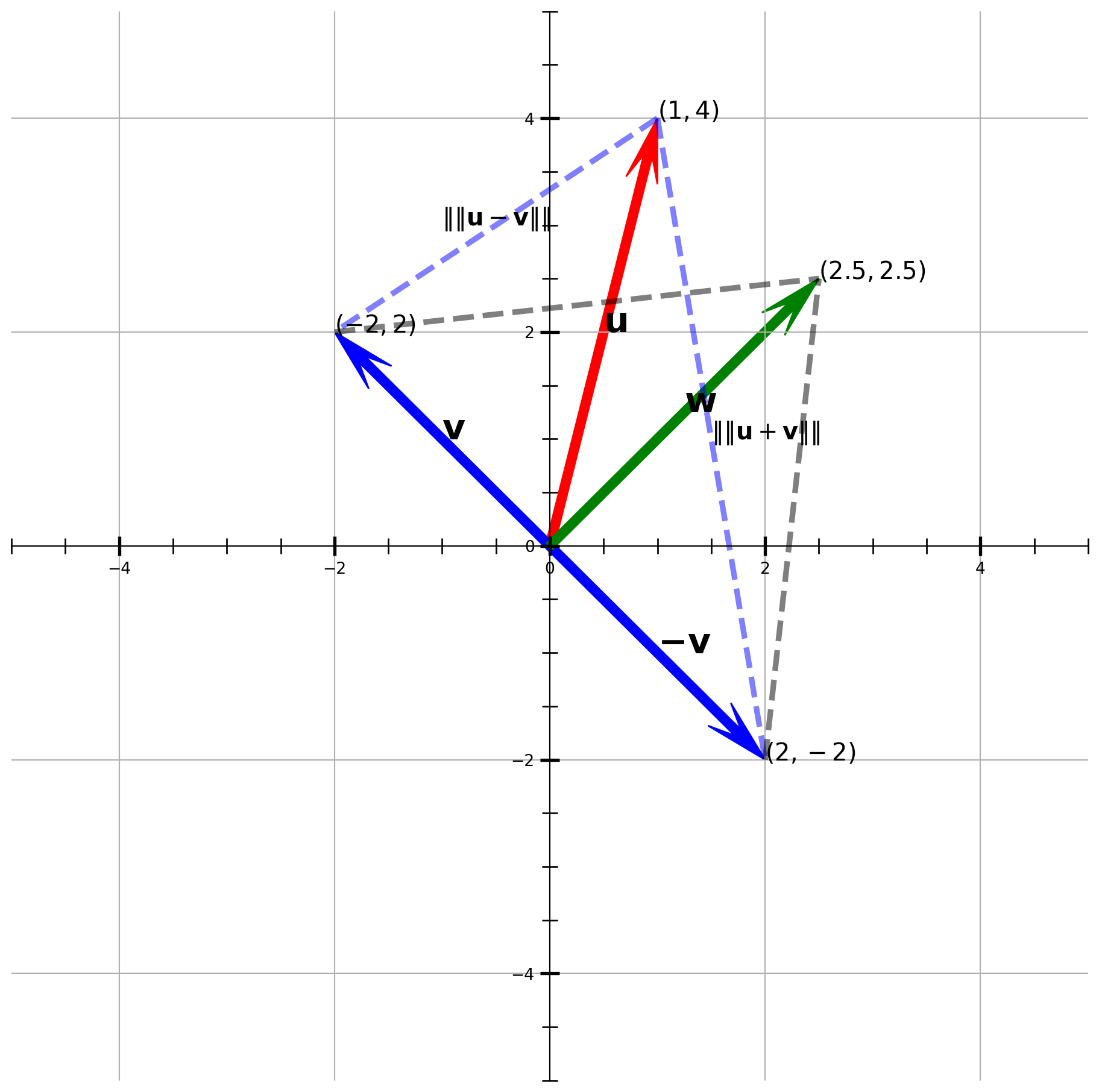

Use SciPy built-in function, construct two $2\times 2$ matrices for holding head and tail coordinates of the vector.

a = np.array([[1, 4], [-2, 2]])
b = np.array([[1, 4], [2, -2]])

distance = sp.spatial.distance.pdist(a, "euclidean")
distance

array([3.60555128])

distance = sp.spatial.distance.pdist(b, "euclidean")
distance

array([6.08276253])

Verify by NumPy .norm.

def dist(u, v):
    a = np.linalg.norm(u - v)
    return a

u = np.array([1, 4])
v = np.array([-2, 2])
dist(u, v)

$\displaystyle 3.60555127546399$

u = np.array([1, 4])
v = np.array([2, -2])
dist(u, v)

$\displaystyle 6.08276253029822$

Now Let’s test if vector $(2.5, 2.5)^T$ is perpendicular to $(2, -2)^T$ and $(-2, 2)^T$.

a = np.array([[2.5, 2.5], [-2, 2]])
b = np.array([[2.5, 2.5], [2, -2]])
distance1 = sp.spatial.distance.pdist(a, "euclidean")
distance2 = sp.spatial.distance.pdist(b, "euclidean")

print(distance1, distance2)

[4.52769257] [4.52769257]

They are the same length, which means $\mathbf{w}\perp \mathbf{v}$ and $\mathbf{w}\perp \mathbf{-v}$.

Orthogonal Complements

In general, the set of all vectors $\mathbf{z}$ that are orthogonal to subspace $W$ is called orthogonal complement, or denoted as $W^\perp$.

The most common example would be

\[(\operatorname{Row} A)^{\perp}=\operatorname{Nul} A \quad \text { and } \quad(\operatorname{Col} A)^{\perp}=\operatorname{Nul} A^{T}\]

The nullspace of $A$ is perpendicular to the row space of $A$; the nullspace of $A^T$ is perpendicular to the column space of $A$.

Angles in $\mathbb{R}^n$

Here is the formula of calculating angles in vector space, to derive it we need the law of cosine:

\[\|\mathbf{u}-\mathbf{v}\|^{2}=\|\mathbf{u}\|^{2}+\|\mathbf{v}\|^{2}-2\|\mathbf{u}\|\|\mathbf{v}\| \cos \vartheta\]

Rearrange, we get

\[\begin{aligned} \|\mathbf{u}\|\|\mathbf{v}\| \cos \vartheta &=\frac{1}{2}\left[\|\mathbf{u}\|^{2}+\|\mathbf{v}\|^{2}-\|\mathbf{u}-\mathbf{v}\|^{2}\right] \\ &=\frac{1}{2}\left[u_{1}^{2}+u_{2}^{2}+v_{1}^{2}+v_{2}^{2}-\left(u_{1}-v_{1}\right)^{2}-\left(u_{2}-v_{2}\right)^{2}\right] \\ &=u_{1} v_{1}+u_{2} v_{2} \\ &=\mathbf{u} \cdot \mathbf{v} \end{aligned}\]

In statistics, $\cos{\vartheta}$ is called correlation coefficient.

\[ \cos{\vartheta}=\frac{\mathbf{u} \cdot \mathbf{v}}{\|\mathbf{u}\|\|\mathbf{v}\|} \]

Geometric Interpretation of Dot Product

You may have noticed that the terms dot product and inner product are sometimes used interchangeably. However, they have distinct meanings.

Functions and polynomials can also have an inner product, but we typically use the term dot product to refer to the inner product within vector spaces.

The dot product has an interesting geometric interpretation. Consider two vectors, $\mathbf{a}$ and $\mathbf{u}$, pointing in different directions, with an angle $\vartheta$ between them. Suppose $\mathbf{u}$ is a unit vector. We want to determine how much $\mathbf{a}$ is aligned with the direction of $\mathbf{u}$.

This value can be calculated by projecting $\mathbf{a}$ onto $\mathbf{u}$:

\[ \|\mathbf{a}\|\cos{\vartheta} = \|\mathbf{a}\| \|\mathbf{u}\|\cos{\vartheta} = \mathbf{a} \cdot \mathbf{u} \]

Any vector $\mathbf{b}$ can be normalized to a unit vector $\mathbf{u}$. By performing the calculation above, we can determine how much $\mathbf{b}$ is aligned with the direction of $\mathbf{u}$.

Orthogonal Sets

If a set of vectors $S = \left\{\mathbf{u}_{1}, \ldots, \mathbf{u}_{p}\right\}$ in $\mathbb{R}^{n}$ has any arbitrary pair to be orthogonal, i.e. $\mathbf{u}_{i} \cdot \mathbf{u}_{j}=0$ whenever $i \neq j$, $S =\left\{\mathbf{u}_{1}, \ldots, \mathbf{u}_{p}\right\}$ is called an orthogonal set.

Naturally, orthogonal set $S$ is linearly independent, they are also an orthogonal basis for space spanned by $\left\{\mathbf{u}_{1}, \ldots, \mathbf{u}_{p}\right\}$. Orthogonal basis has an advantage is that coordinates of the basis can be quickly computed.

For instance any $\mathbf{y}$ in $W$,

\[ \mathbf{y}=c_{1} \mathbf{u}_{1}+\cdots+c_{p} \mathbf{u}_{p} \]

Because it is an orthogonal sets,

\[ \mathbf{y} \cdot \mathbf{u}_{1}=\left(c_{1} \mathbf{u}_{1}+c_{2} \mathbf{u}_{2}+\cdots+c_{p} \mathbf{u}_{p}\right) \cdot \mathbf{u}_{1}=c_{1}\left(\mathbf{u}_{1} \cdot \mathbf{u}_{1}\right) \]

Thus

\[c_{j}=\frac{\mathbf{y} \cdot \mathbf{u}_{j}}{\mathbf{u}_{j} \cdot \mathbf{u}_{j}} \quad(j=1, \ldots, p)\]

Orthogonal Projection

For any $\mathbf{y}$ in $\mathbb{R}^n$, we want to decompose it as

\[ \mathbf{y} = \alpha \mathbf{u}+\mathbf{z} = \hat{\mathbf{y}}+\mathbf{z} \]

where $ $ is perpendicular to $\mathbf{z}$, $\alpha$ is a scalar.And the subspace $L$ spanned by $\mathbf{u}$, the projection of $\mathbf{y}$ onto $L$ is denoted as

\[\hat{\mathbf{y}}=\operatorname{proj}_{L} \mathbf{y}=\frac{\mathbf{y} \cdot \mathbf{u}}{\mathbf{u} \cdot \mathbf{u}} \mathbf{u}\]

Becasue $\mathbf{u}\perp \mathbf{z}$, then $\mathbf{u}\cdot \mathbf{z} = 0$, replace $\mathbf{z}$ by $\mathbf{y}- \alpha \mathbf{u}$:

\[ (\mathbf{y}- \alpha \mathbf{u})\cdot \mathbf{u}= 0\\ \alpha = \frac{\mathbf{y}\cdot \mathbf{u}}{\mathbf{u}\cdot \mathbf{u}} \]

Now we get the formula for projection onto $L$ spanned by $\mathbf{u}$.

A Visual Example in $\mathbb{R}^T$

Suppose we have $\mathbf{y} = (2, 5)^T$, $\mathbf{u} = (3, 1)^T$. Plot $\hat{\mathbf{y}}$ onto the subspace spanned $L$ by $\mathbf{u}$.

fig, ax = plt.subplots(figsize=(12, 12))

vects = np.array([[4, 5], [2, 1]])
colr = ["red", "blue"]
cordt = ["$(4, 5)$", "$(2, 1)$"]
vec_name = [r"$\mathbf{y}$", r"$\mathbf{u}$"]

for i in range(2):
    ax.arrow(
        0,
        0,
        vects[i][0],
        vects[i][1],
        color=colr[i],
        width=0.03,
        length_includes_head=True,
        head_width=0.1,  # default: 3*width
        head_length=0.2,
        overhang=0.4,
    )
    ax.text(
        x=vects[i][0],
        y=vects[i][1],
        s=cordt[i],
        size=15,
        color=colr[i],
        verticalalignment="bottom",
    )
    ax.text(
        x=vects[i][0] / 2,
        y=vects[i][1] / 2,
        s=vec_name[i],
        size=22,
        color=colr[i],
        verticalalignment="bottom",
    )

################################### Subspace L ############################
x = np.linspace(0, 8.1, 100)
y = 1 / 2 * x
ax.plot(x, y, lw=3, color="red", alpha=0.5)
ax.text(x=6.5, y=3, s=r"$L = \operatorname{Span}(\mathbf{u})$", size=19, color="red")

ax.axis([0, 8, 0, 8])
ax.grid()

plt.show()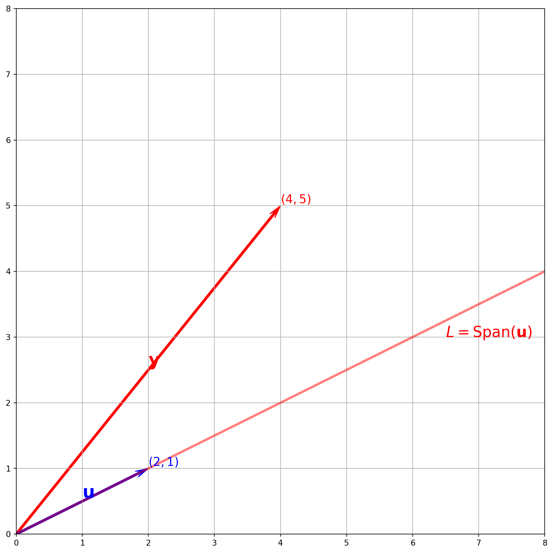

Let’s use formula to compute $\alpha$ and $\hat{\mathbf{y}}$.

y = np.array([4, 5])
u = np.array([2, 1])
alpha = (y @ u) / (u @ u)
alpha

$\displaystyle 2.6$

yhat = alpha * u
yhat

array([5.2, 2.6])

With results above, we can plot the orthogonal projection.

fig, ax = plt.subplots(figsize=(12, 12))

vects = np.array([[4, 5], [2, 1], [5.2, 2.6]])
colr = ["red", "blue", "green"]
cordt = ["$(4, 5)$", "$(2, 1)$", r"$(5.2, 2.6)$"]
vec_name = [r"$\mathbf{y}$", r"$\mathbf{u}$", r"$\hat{\mathbf{y}} = \alpha\mathbf{u}$"]

for i in range(3):
    ax.arrow(
        0,
        0,
        vects[i][0],
        vects[i][1],
        color=colr[i],
        width=0.03,
        length_includes_head=True,
        head_width=0.1,  # default: 3*width
        head_length=0.2,
        overhang=0.4,
        zorder=-i,
    )
    ax.text(x=vects[i][0], y=vects[i][1], s=cordt[i], size=19)
    ax.text(x=vects[i][0] / 2, y=vects[i][1] / 2, s=vec_name[i], size=22)

##################################### Components of y orthogonal to u ##########################

point1 = [4, 5]
point2 = [5.2, 2.6]
line1 = np.array([point1, point2])
ax.plot(line1[:, 0], line1[:, 1], c="k", lw=3.5, alpha=0.5, ls="--")
ax.text(4.7, 3.8, r"$\mathbf{z}$", size=22)

################################### Subspace L ############################
x = np.linspace(0, 8.1, 100)
y = 0.5 * x
ax.plot(x, y, lw=3, color="red", alpha=0.5, zorder=-3)
ax.text(x=6.5, y=3, s=r"$L = \operatorname{Span}(\mathbf{u})$", size=19)

ax.axis([0, 8, 0, 8])
ax.grid()

#################################### Formula ################################
ax.text(
    x=1,
    y=7,
    s=r"$(\mathbf{y} - \alpha \mathbf{u}) \cdot \mathbf{u} = 0$",
    size=22,
    color="b",
)
ax.text(
    x=1,
    y=6.5,
    s=r"$\alpha = \frac{\mathbf{y} \cdot \mathbf{u}}{\mathbf{u} \cdot \mathbf{u}}$",
    size=22,
    color="b",
)
ax.text(
    x=1,
    y=6,
    s=r"$\operatorname{proj}_{L} \mathbf{y} = \frac{\mathbf{y} \cdot \mathbf{u}}{\mathbf{u} \cdot \mathbf{u}} \mathbf{u}$",
    size=22,
    color="b",
)

plt.show()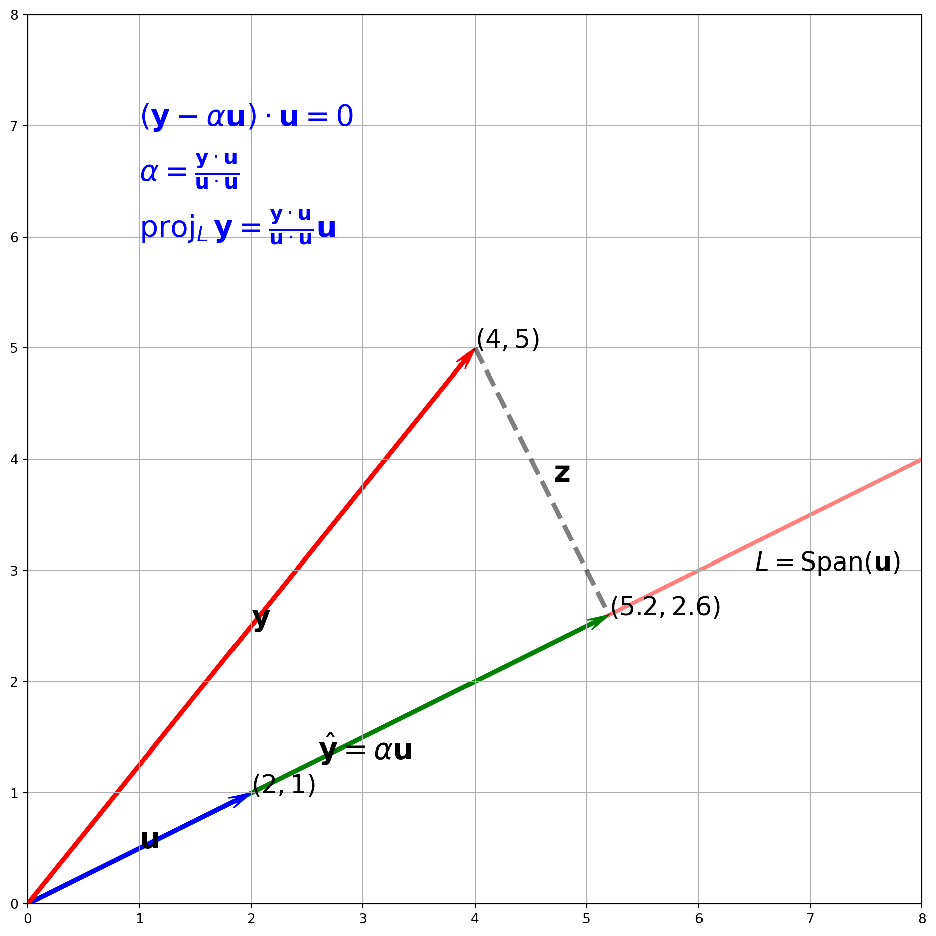

The Orthogonal Decomposition Theorem

To generalize the orthogonal projection in the higher dimension $\mathbb{R}^n$, we summarize the idea into the orthogonal decomposition theorem.

Let $W$ be a subspace of $\mathbb{R}^{n}$. Then each $\mathbf{y}$ in $\mathbb{R}^{n}$ can be written uniquely in the form \[ \mathbf{y}=\hat{\mathbf{y}}+\mathbf{z} \] where $\hat{\mathbf{y}}$ is in $W$ and $\mathbf{z}$ is in $W^{\perp} .$ In fact, if $\left\{\mathbf{u}_{1}, \ldots, \mathbf{u}_{p}\right\}$ is any orthogonal basis of $W,$ then \[ \hat{\mathbf{y}}=\frac{\mathbf{y} \cdot \mathbf{u}_{1}}{\mathbf{u}_{1} \cdot \mathbf{u}_{1}} \mathbf{u}_{1}+\cdots+\frac{\mathbf{y} \cdot \mathbf{u}_{p}}{\mathbf{u}_{p} \cdot \mathbf{u}_{p}} \mathbf{u}_{p} \] and $\mathbf{z}=\mathbf{y}-\hat{\mathbf{y}}$.

In $\mathbb{R}^{2}$, we project $\mathbf{y}$ onto subspace $L$ which is spanned by $\mathbf{u}$, here we generalize the formula for $\mathbb{R}^{n}$, that $\mathbf{y}$ is projected onto $W$ which is spanned by $\left\{\mathbf{u}_{1}, \ldots, \mathbf{u}_{p}\right\}$.

A Visual Example in $\mathbb{R}^{3}$

A subspace $W=\operatorname{Span}\left\{\mathbf{u}_{1}, \mathbf{u}_{2}\right\}$, and a vector $\mathbf{y}$ is not in $W$, decompose $\mathbf{y}$ into $\hat{\mathbf{y}} + \mathbf{z}$, and plot them.

where

\[\mathbf{u}_{1}=\left[\begin{array}{r} 2 \\ 5 \\ -1 \end{array}\right], \mathbf{u}_{2}=\left[\begin{array}{r} -2 \\ 1 \\ 1 \end{array}\right], \text { and } \mathbf{y}=\left[\begin{array}{l} 1 \\ 2 \\ 3 \end{array}\right]\]

The projection onto $W$ in $\mathbb{R}^3$ is

\[ \hat{\mathbf{y}}=\frac{\mathbf{y} \cdot \mathbf{u}_{1}}{\mathbf{u}_{1} \cdot \mathbf{u}_{1}} \mathbf{u}_{1}+\frac{\mathbf{y} \cdot \mathbf{u}_{2}}{\mathbf{u}_{2} \cdot \mathbf{u}_{2}} \mathbf{u}_{2}=\hat{\mathbf{y}}_{1}+\hat{\mathbf{y}}_{2} \]

The codes for plotting are quite redundent, however exceedingly intuitive.

######################## Subspace W ##############################
s = np.linspace(-0.5, 0.5, 10)
t = np.linspace(-0.5, 0.5, 10)
S, T = np.meshgrid(s, t)

X1 = 2 * S - 2 * T
X2 = 5 * S + T
X3 = -S + T

fig = plt.figure(figsize=(7, 7))
ax = fig.add_subplot(projection="3d")
ax.plot_wireframe(X1, X2, X3, linewidth=1.5, alpha=0.3)

########################### Vector y ###############################
y = np.array([1, 2, 3])
u1, u2 = np.array([2, 5, -1]), np.array([-2, 1, 1])

vec = np.array([[0, 0, 0, y[0], y[1], y[2]]])
X, Y, Z, U, V, W = zip(*vec)
ax.quiver(
    X,
    Y,
    Z,
    U,
    V,
    W,
    length=1,
    normalize=False,
    color="red",
    alpha=0.6,
    arrow_length_ratio=0.08,
    pivot="tail",
    linestyles="solid",
    linewidths=3,
)

ax.text(y[0], y[1], y[2], r"$\mathbf{y}$", size=15)
########################### Vector u1 and u2 ###############################

vec = np.array([[0, 0, 0, u1[0], u1[1], u1[2]]])
X, Y, Z, U, V, W = zip(*vec)
ax.quiver(
    X,
    Y,
    Z,
    U,
    V,
    W,
    length=1,
    normalize=False,
    color="red",
    alpha=0.6,
    arrow_length_ratio=0.08,
    pivot="tail",
    linestyles="solid",
    linewidths=3,
)

vec = np.array([[0, 0, 0, u2[0], u2[1], u2[2]]])
X, Y, Z, U, V, W = zip(*vec)
ax.quiver(
    X,
    Y,
    Z,
    U,
    V,
    W,
    length=1,
    normalize=False,
    color="red",
    alpha=0.6,
    arrow_length_ratio=0.08,
    pivot="tail",
    linestyles="solid",
    linewidths=3,
)


ax.text(u1[0], u1[1], u1[2], r"$\mathbf{u}_1$", size=15)
ax.text(u2[0], u2[1], u2[2], r"$\mathbf{u}_2$", size=15)
########################### yhat ###############################

alpha1 = (y @ u1) / (u1 @ u1)
alpha2 = (y @ u2) / (u2 @ u2)

yhat1 = alpha1 * u1
yhat2 = alpha2 * u2
yhat = yhat1 + yhat2

vec = np.array([[0, 0, 0, yhat1[0], yhat1[1], yhat1[2]]])
X, Y, Z, U, V, W = zip(*vec)
ax.quiver(
    X,
    Y,
    Z,
    U,
    V,
    W,
    length=1,
    normalize=False,
    color="blue",
    alpha=0.6,
    arrow_length_ratio=0.08,
    pivot="tail",
    linestyles="solid",
    linewidths=3,
    zorder=3,
)

vec = np.array([[0, 0, 0, yhat2[0], yhat2[1], yhat2[2]]])
X, Y, Z, U, V, W = zip(*vec)
ax.quiver(
    X,
    Y,
    Z,
    U,
    V,
    W,
    length=1,
    normalize=False,
    color="blue",
    alpha=0.6,
    arrow_length_ratio=0.08,
    pivot="tail",
    linestyles="solid",
    linewidths=3,
    zorder=3,
)

vec = np.array([[0, 0, 0, yhat[0], yhat[1], yhat[2]]])
X, Y, Z, U, V, W = zip(*vec)
ax.quiver(
    X,
    Y,
    Z,
    U,
    V,
    W,
    length=1,
    normalize=False,
    color="pink",
    alpha=1,
    arrow_length_ratio=0.12,
    pivot="tail",
    linestyles="solid",
    linewidths=3,
    zorder=3,
)

ax.text(yhat1[0], yhat1[1], yhat1[2], r"$\hat{\mathbf{y}}_1$", size=15)
ax.text(yhat2[0], yhat2[1], yhat2[2], r"$\hat{\mathbf{y}}_2$", size=15)
ax.text(
    x=yhat[0],
    y=yhat[1],
    z=yhat[2],
    s=r"$\hat{\mathbf{y}}=\frac{\mathbf{y} \cdot \mathbf{u}_{1}}{\mathbf{u}_{1} \cdot \mathbf{u}_{1}} \mathbf{u}_{1}+\frac{\mathbf{y} \cdot \mathbf{u}_{2}}{\mathbf{u}_{2} \cdot \mathbf{u}_{2}} \mathbf{u}_{2}=\hat{\mathbf{y}}_{1}+\hat{\mathbf{y}}_{2}$",
    size=15,
)
########################### z ###############################
z = y - yhat
vec = np.array([[yhat[0], yhat[1], yhat[2], z[0], z[1], z[2]]])
X, Y, Z, U, V, W = zip(*vec)
ax.quiver(
    X,
    Y,
    Z,
    U,
    V,
    W,
    length=1,
    normalize=False,
    color="green",
    alpha=0.6,
    arrow_length_ratio=0.08,
    pivot="tail",
    linestyles="solid",
    linewidths=3,
)

############################ Dashed Line ####################

line1 = np.array([y, yhat1])
ax.plot(line1[:, 0], line1[:, 1], line1[:, 2], c="b", lw=3.5, alpha=0.5, ls="--")

line2 = np.array([y, yhat2])
ax.plot(line2[:, 0], line2[:, 1], line2[:, 2], c="b", lw=2.5, alpha=0.5, ls="--")

line3 = np.array([yhat, yhat2])
ax.plot(line3[:, 0], line3[:, 1], line3[:, 2], c="b", lw=2.5, alpha=0.5, ls="--")

line4 = np.array([yhat, yhat1])
ax.plot(line4[:, 0], line4[:, 1], line4[:, 2], c="b", lw=2.5, alpha=0.5, ls="--")

############################# View Angle
ax.view_init(elev=-6, azim=12)

plt.show()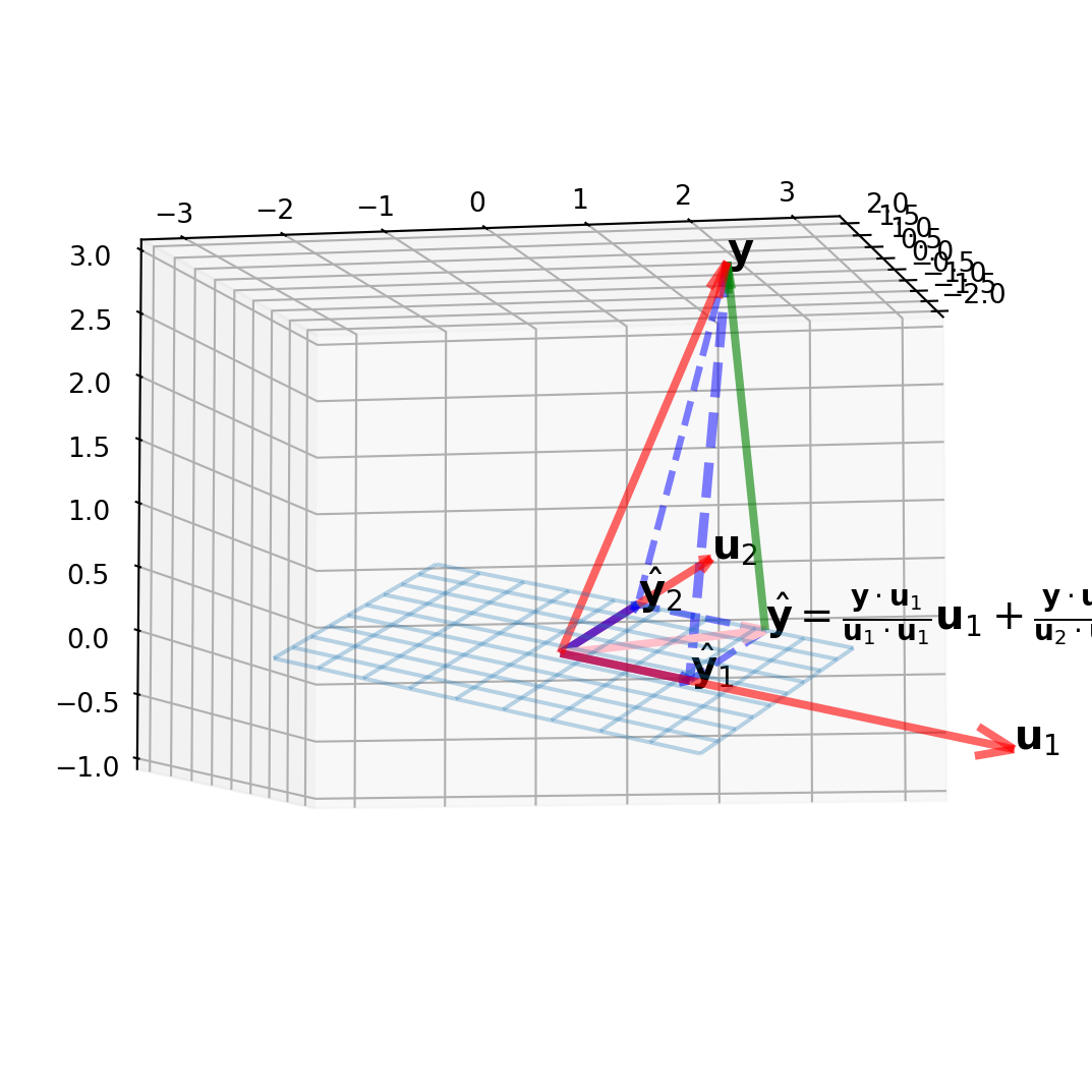

Orthonormal Sets

An orthonormal set is obtained from normalizing the orthogonal set, and also called orthonomal basis.

Matrices whose columns form an orthonormal set are important for matrix computation.

Let $U=\left[\begin{array}{lll} \mathbf{u}_{1} & \mathbf{u}_{2} & \mathbf{u}_{3} \end{array}\right]$, where $\mathbf{u}_{i}$’s are from an orthonormal set, the outer product, $U^TU$ is

\[U^{T} U=\left[\begin{array}{l} \mathbf{u}_{1}^{T} \\ \mathbf{u}_{2}^{T} \\ \mathbf{u}_{3}^{T} \end{array}\right]\left[\begin{array}{lll} \mathbf{u}_{1} & \mathbf{u}_{2} & \mathbf{u}_{3} \end{array}\right]=\left[\begin{array}{lll} \mathbf{u}_{1}^{T} \mathbf{u}_{1} & \mathbf{u}_{1}^{T} \mathbf{u}_{2} & \mathbf{u}_{1}^{T} \mathbf{u}_{3} \\ \mathbf{u}_{2}^{T} \mathbf{u}_{1} & \mathbf{u}_{2}^{T} \mathbf{u}_{2} & \mathbf{u}_{2}^{T} \mathbf{u}_{3} \\ \mathbf{u}_{3}^{T} \mathbf{u}_{1} & \mathbf{u}_{3}^{T} \mathbf{u}_{2} & \mathbf{u}_{3}^{T} \mathbf{u}_{3} \end{array}\right]\]

And $\mathbf{u}_{i}^{T} \mathbf{u}_{j}, i, j \in (1, 2, 3)$ is an inner product.

Because of orthonormal sets, we have

\[ \mathbf{u}_{1}^{T} \mathbf{u}_{2}=\mathbf{u}_{2}^{T} \mathbf{u}_{1}=0, \quad \mathbf{u}_{1}^{T} \mathbf{u}_{3}=\mathbf{u}_{3}^{T} \mathbf{u}_{1}=0, \quad \mathbf{u}_{2}^{T} \mathbf{u}_{3}=\mathbf{u}_{3}^{T} \mathbf{u}_{2}=0\\ \mathbf{u}_{1}^{T} \mathbf{u}_{1}=1, \quad \mathbf{u}_{2}^{T} \mathbf{u}_{2}=1, \quad \mathbf{u}_{3}^{T} \mathbf{u}_{3}=1 \]

which means

\[ U^TU = I \]

Recall that we have a general projection formula

\[ \hat{\mathbf{y}}=\frac{\mathbf{y} \cdot \mathbf{u}_{1}}{\mathbf{u}_{1} \cdot \mathbf{u}_{1}} \mathbf{u}_{1}+\cdots+\frac{\mathbf{y} \cdot \mathbf{u}_{p}}{\mathbf{u}_{p} \cdot \mathbf{u}_{p}} \mathbf{u}_{p} =\frac{\mathbf{y} \cdot \mathbf{u}_{1}}{{\mathbf{u}_{1}^T} \mathbf{u}_{1}} \mathbf{u}_{1}+\cdots+\frac{\mathbf{y} \cdot \mathbf{u}_{p}}{{\mathbf{u}_{p}^T} \mathbf{u}_{p}} \mathbf{u}_{p}\\ \]

If the $\{\mathbf{u}_1,...,\mathbf{u}_p\}$ is an orthonormal set, then

\[\begin{align} \hat{\mathbf{y}}&=\left(\mathbf{y} \cdot \mathbf{u}_{1}\right) \mathbf{u}_{1}+\left(\mathbf{y} \cdot \mathbf{u}_{2}\right) \mathbf{u}_{2}+\cdots+\left(\mathbf{y} \cdot \mathbf{u}_{p}\right) \mathbf{u}_{p}\\ & = \left(\mathbf{u}_{1}^T\mathbf{y}\right) \mathbf{u}_{1}+\left(\mathbf{u}_{2}^T\mathbf{y}\right) \mathbf{u}_{2}+\cdots+\left(\mathbf{u}_{p}^T\mathbf{y}\right) \mathbf{u}_{p}\\ \end{align}\]

Cross Product

This is the formula of Cross product \[ \mathbf{a} \times \mathbf{b}=\|\mathbf{a}\|\|\mathbf{b}\| \sin (\theta) \mathbf{n} \] The output of cross product is the length of vector $\mathbf{c}$ which is perpendicular to both $ $ and $ $.

# Define the two vectors
a = np.array([5, 2, 3])
b = np.array([4, 8, 10])

# Calculate the cross product
c = np.cross(a, b)

# Create the 3D plot
fig = go.Figure(
    data=[
        go.Scatter3d(
            x=[0, a[0]],
            y=[0, a[1]],
            z=[0, a[2]],
            mode="lines",
            name="Vector a",
            line=dict(color="red", width=5),
        ),
        go.Scatter3d(
            x=[0, b[0]],
            y=[0, b[1]],
            z=[0, b[2]],
            mode="lines",
            name="Vector b",
            line=dict(color="green", width=5),
        ),
        go.Scatter3d(
            x=[0, c[0]],
            y=[0, c[1]],
            z=[0, c[2]],
            mode="lines",
            name="Vector c (cross product)",
            line=dict(color="blue", width=5),
        ),
    ]
)

# Set the axis labels
fig.update_layout(scene=dict(xaxis_title="X", yaxis_title="Y", zaxis_title="Z"))

# Show the plot
fig.show()

The Dot Product

The Norm of a Vector

Distance in \(\mathbb{R}^n\)