import matplotlib.pyplot as plt
import numpy as np
import sympy as sy

sy.init_printing()

def round_expr(expr, num_digits):
    return expr.xreplace({n: round(n, num_digits) for n in expr.atoms(sy.Number)})

In time series analysis, we study difference equations by writing them into a linear system. For instance,

\[ 3y_{t+3} - 2y_{t+2} + 4y_{t+1} - y_t = 0 \]

We define

\[ \mathbf{x}_t = \left[ \begin{matrix} y_t\\ y_{t+1}\\ y_{t+2} \end{matrix} \right], \qquad \mathbf{x}_{t+1} = \left[ \begin{matrix} y_{t+1}\\ y_{t+2}\\ y_{t+3} \end{matrix} \right] \]

Rerrange the difference equation for better visual representation,

\[ y_{t+3} = \frac{2}{3}y_{t+2} - \frac{4}{3}y_{t+1} + \frac{1}{3}y_{t} \]

The difference equation can be rewritten as

\[ \mathbf{x}_{t+1} = A \mathbf{x}_{t} \]

That is,

\[ \left[ \begin{matrix} y_{t+1}\\ y_{t+2}\\ y_{t+3} \end{matrix} \right] = \left[ \begin{matrix} 0 & 1 & 0\\ 0 & 0 & 1\\ \frac{1}{3} & -\frac{4}{3} & \frac{2}{3} \end{matrix} \right] \left[ \begin{matrix} y_t\\ y_{t+1}\\ y_{t+2} \end{matrix} \right] \]

In general, we make sure the difference equation look like:

\[ y_{t+k} = a_1y_{t+k-1} + a_2y_{t+k-2} + ... + a_ky_{t} \]

then rewrite as \(\mathbf{x}_{t+1} = A \mathbf{x}_{t}\), where

\[ \mathbf{x}_t = \left[ \begin{matrix} y_{t}\\ y_{t+1}\\ \vdots\\ y_{t+k-1} \end{matrix} \right], \quad \mathbf{x}_{t+1} = \left[ \begin{matrix} y_{t+1}\\ y_{t+2}\\ \vdots\\ y_{t+k} \end{matrix} \right] \]

And also

\[A=\left[\begin{array}{ccccc} 0 & 1 & 0 & \cdots & 0 \\ 0 & 0 & 1 & & 0 \\ \vdots & & & \ddots & \vdots \\ 0 & 0 & 0 & & 1 \\ a_{k} & a_{k-1} & a_{k-2} & \cdots & a_{1} \end{array}\right]\]

Markov Chains

Markov chain is a type of stochastic process, commonly modeled by difference equation, we will be slightly touching the surface of this topic by walking through an example.

Markov chain is also described by the first-order difference equation \(\mathbf{x}_{t+1} = P\mathbf{x}_t\), where \(\mathbf{x}_t\) is called state vector, \(A\) is called stochastic matrix.

Suppose there are 3 cities \(A\), \(B\) and \(C\), the proportion of population migration among cities are constructed in the stochastic matrix below

\[ M = \left[ \begin{matrix} .89 & .07 & .10\\ .07 & .90 & .11\\ .04 & .03 & .79 \end{matrix} \right] \]

For instance, the first column means that \(89\%\) of population will stay in city \(A\), \(7\%\) will move to city \(B\) and \(4\%\) will migrate to city \(C\). The first row means \(7\%\) of city \(B\)’s population will immigrate into \(A\), \(10\%\) of city \(C\)’s population will immigrate into \(A\).

Suppose the initial population of 3 cities are \((593000, 230000, 709000)\), convert the entries into percentage of total population.

x = np.array([593000, 230000, 709000])
x = x / np.sum(x)
x

array([0.38707572, 0.15013055, 0.46279373])

Input the stochastic matrix

M = np.array([[0.89, 0.07, 0.1], [0.07, 0.9, 0.11], [0.04, 0.03, 0.79]])

After the first period, the population proportion among cities are

x1 = M @ x
x1

array([0.4012859 , 0.2131201 , 0.38559399])

The second period

x2 = M @ x1
x2

array([0.41062226, 0.26231345, 0.3270643 ])

The third period

x3 = M @ x2
x3

array([0.41652218, 0.30080273, 0.28267509])

We can construct a loop till \(\mathbf{x}_{100} = M\mathbf{x}_{99}\), then plot the dynamic path. Notice that the curve is flattening after 20 periods, and we call it convergence to steady-state.

k = 100
X = np.zeros((k, 3))
X[0] = M @ x
i = 0

while i + 1 < 100:
    X[i + 1] = M @ X[i]
    i = i + 1

fig, ax = plt.subplots(figsize=(12, 12))

la = ["City A", "City B", "City C"]
s = "$%.3f$"
for i in [0, 1, 2]:
    ax.plot(X[:, i], lw=3, label=la[i])
    ax.text(x=20, y=X[-1, i], s=s % X[-1, i], size=16)

ax.axis(
    [0, 20, 0, 0.6]
)  # No need to show more of x, it reaches steady-state around 20 periods
ax.legend(fontsize=16)
ax.grid()
ax.set_title("Dynamics of Population Percentage")
plt.show()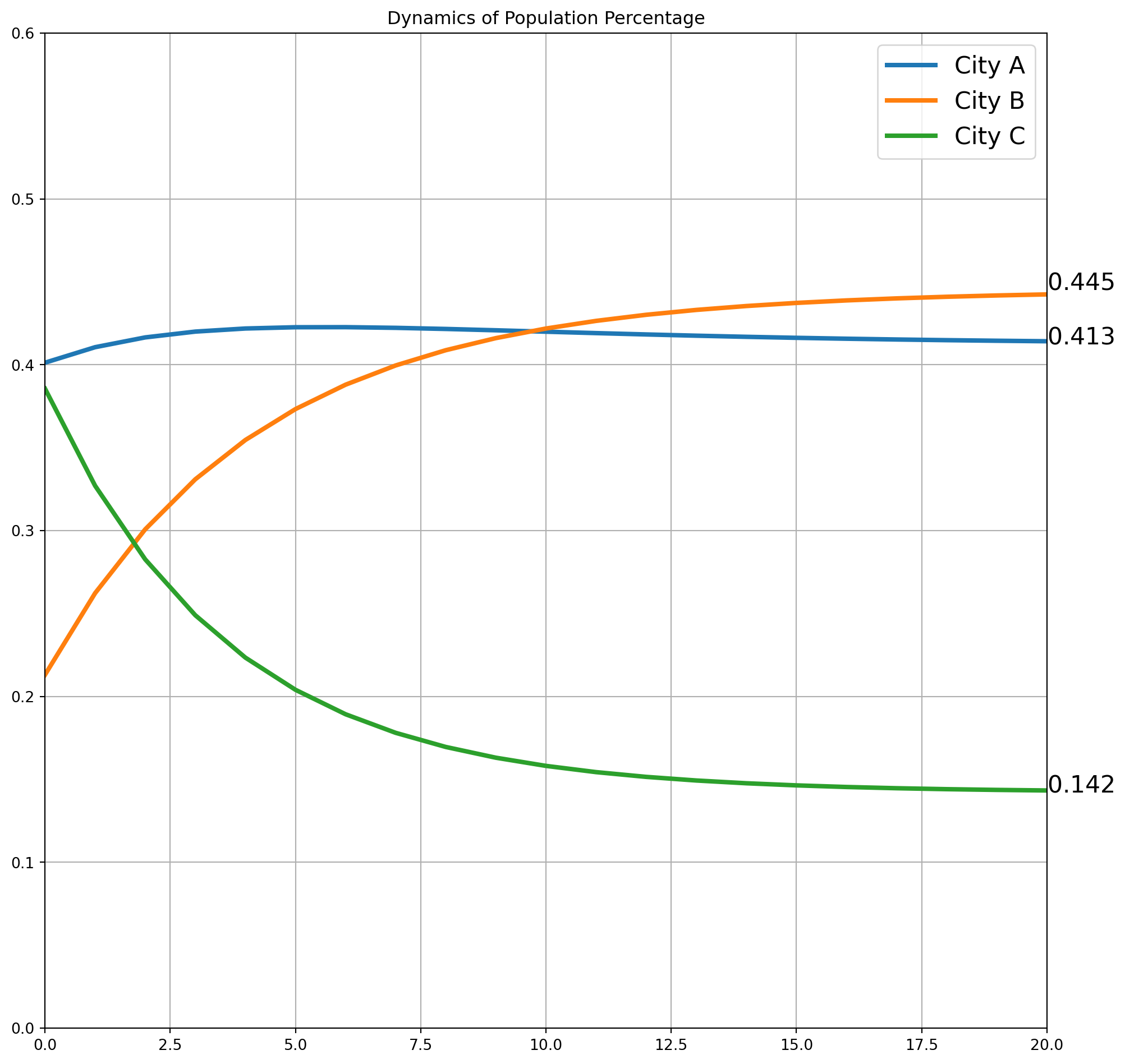

Eigenvalue and -vector in Markov Chain

If the \(M\) in last example is diagonalizable, there will be \(n\) linearly independent eigenvectors and corresponding eigenvalues, \(\lambda_1\),…,\(\lambda_n\). And eigenvalues can always be arranged so that \(\left|\lambda_{1}\right| \geq\left|\lambda_{2}\right| \geq \cdots \geq\left|\lambda_{n}\right|\).

Also, because any initial vector \(\mathbb{x}_0 \in \mathbb{R}^n\), we can use the basis of eigenspace (eigenvectors) to represent all \(\mathbf{x}\).

\[ \mathbf{x}_{0}=c_{1} \mathbf{v}_{1}+\cdots+c_{n} \mathbf{v}_{n} \]

This is called eigenvector decomposition of \(\mathbf{x}_0\). Multiply by \(A\)

\[ \begin{aligned} \mathbf{x}_{1}=A \mathbf{x}_{0} &=c_{1} A \mathbf{v}_{1}+\cdots+c_{n} A \mathbf{v}_{n} \\ &=c_{1} \lambda_{1} \mathbf{v}_{1}+\cdots+c_{n} \lambda_{n} \mathbf{v}_{n} \end{aligned} \]

In general, we have a formula for \(\mathbf{x}_k\)

\[ \mathbf{x}_{k}=c_{1}\left(\lambda_{1}\right)^{k} \mathbf{v}_{1}+\cdots+c_{n}\left(\lambda_{n}\right)^{k} \mathbf{v}_{n} \]

Now we test if \(M\) has \(n\) linearly independent eigvectors.

M = sy.Matrix([[0.89, 0.07, 0.1], [0.07, 0.9, 0.11], [0.04, 0.03, 0.79]])
M

\(\displaystyle \left[\begin{matrix}0.89 & 0.07 & 0.1\\0.07 & 0.9 & 0.11\\0.04 & 0.03 & 0.79\end{matrix}\right]\)

M.is_diagonalizable()

True

\(M\) is diagonalizable, which also means that \(M\) has \(n\) linearly independent eigvectors.

P, D = M.diagonalize()
P = round_expr(P, 4)
P  # user-defined round function at the top of the notebook

\(\displaystyle \left[\begin{matrix}-0.6618 & -0.6536 & -0.413\\-0.7141 & 0.7547 & -0.4769\\-0.2281 & -0.1011 & 0.89\end{matrix}\right]\)

D = round_expr(D, 4)
D

\(\displaystyle \left[\begin{matrix}1.0 & 0 & 0\\0 & 0.8246 & 0\\0 & 0 & 0.7554\end{matrix}\right]\)

First we find the \(\big[\mathbf{x}_0\big]_C\), i.e. \(c_1, c_2, c_3\)

x0 = sy.Matrix([[0.3870], [0.1501], [0.4627]])
x0

\(\displaystyle \left[\begin{matrix}0.387\\0.1501\\0.4627\end{matrix}\right]\)

P_aug = P.row_join(x0)
P_aug_rref = round_expr(P_aug.rref()[0], 4)
P_aug_rref

\(\displaystyle \left[\begin{matrix}1 & 0 & 0 & -0.6233\\0 & 1 & 0 & -0.1759\\0 & 0 & 1 & 0.3402\end{matrix}\right]\)

c = sy.zeros(3, 1)
for i in [0, 1, 2]:
    c[i] = P_aug_rref[i, 3]
c = round_expr(c, 4)
c

\(\displaystyle \left[\begin{matrix}-0.6233\\-0.1759\\0.3402\end{matrix}\right]\)

Now we can use the formula to compute \(\mathbf{x}_{100}\), it is the same as we have plotted in the graph.

x100 = (
    c[0] * D[0, 0] ** 100 * P[:, 0]
    + c[1] * D[1, 1] ** 100 * P[:, 1]
    + c[2] * D[2, 2] ** 100 * P[:, 2]
)
x100 = round_expr(x100, 4)
x100

\(\displaystyle \left[\begin{matrix}0.4125\\0.4451\\0.1422\end{matrix}\right]\)

This is close enough to the steady-state.

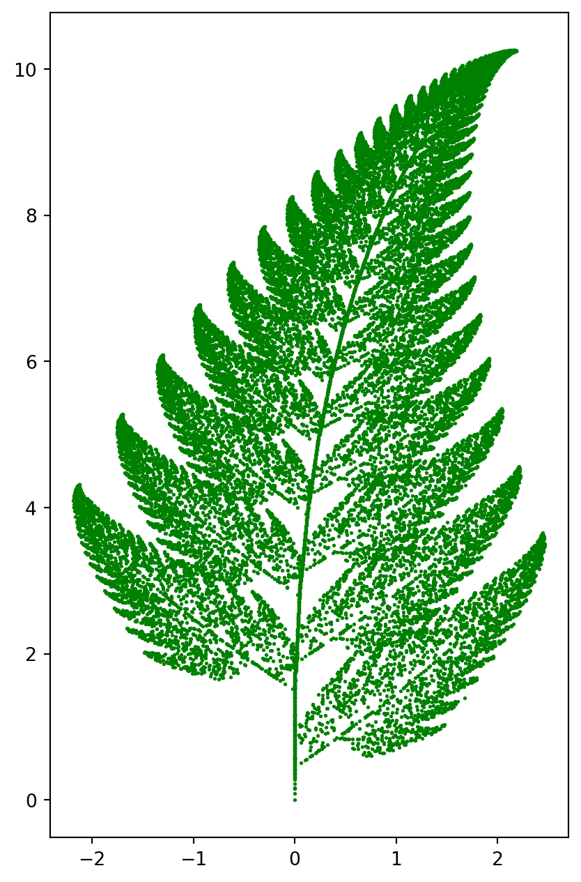
Fractal Pictures

Here is an example of fractal geometry, illustrating how dynamic system and affine transformation can create fractal pictures.

The algorithem is perform 4 types of affine transformation. The corresponding probabilites are \(p_1, p_2, p_3, p_4\).

\[ \begin{array}{l} T_{1}\left(\left[\begin{array}{l} x \\ y \end{array}\right]\right)=\left[\begin{array}{rr} 0.86 & 0.03 \\ -0.03 & 0.86 \end{array}\right]\left[\begin{array}{l} x \\ y \end{array}\right]+\left[\begin{array}{l} 0 \\ 1.5 \end{array}\right], p_{1}=0.83 \\ T_{2}\left(\left[\begin{array}{l} x \\ y \end{array}\right]\right)=\left[\begin{array}{lr} 0.2 & -0.25 \\ 0.21 & 0.23 \end{array}\right]\left[\begin{array}{l} x \\ y \end{array}\right]+\left[\begin{array}{l} 0 \\ 1.5 \end{array}\right], p_{2}=0.09 \\ T_{3}\left(\left[\begin{array}{l} x \\ y \end{array}\right]\right)=\left[\begin{array}{rr} -0.15 & 0.27 \\ 0.25 & 0.26 \end{array}\right]\left[\begin{array}{l} x \\ y \end{array}\right]+\left[\begin{array}{l} 0 \\ 0.45 \end{array}\right], p_{3}=0.07 \\ T_{4}\left(\left[\begin{array}{l} x \\ y \end{array}\right]\right)=\left[\begin{array}{ll} 0 & 0 \\ 0 & 0.17 \end{array}\right]\left[\begin{array}{l} x \\ y \end{array}\right]+\left[\begin{array}{l} 0 \\ 0 \end{array}\right], p_{4}=0.01 \end{array} \]

The codes below are self-explanatory.

A = np.array(
    [
        [[0.86, 0.03], [-0.03, 0.86]],
        [[0.2, -0.25], [0.21, 0.23]],
        [[-0.15, 0.27], [0.25, 0.26]],
        [[0.0, 0.0], [0.0, 0.17]],
    ]
)
a = np.array([[[0, 1.5]], [[0, 1.5]], [[0, 0.45]], [[0, 0]]])

p1 = 1 * np.ones(83)
p2 = 2 * np.ones(9)
p3 = 3 * np.ones(7)
p4 = 4 * np.ones(1)
p = np.hstack((p1, p2, p3, p4))

k = 30000
fig, ax = plt.subplots(figsize=(5, 8))
X = np.zeros((2, k))
for i in range(k - 1):
    n = np.random.randint(0, 100)
    if p[n] == 1:
        X[:, i + 1] = A[0, :, :] @ X[:, i] + a[0, :, :]
    elif p[n] == 2:
        X[:, i + 1] = A[1, :, :] @ X[:, i] + a[1, :, :]
    elif p[n] == 3:
        X[:, i + 1] = A[2, :, :] @ X[:, i] + a[2, :, :]
    else:
        X[:, i + 1] = A[3, :, :] @ X[:, i] + a[3, :, :]
ax.scatter(X[0, :], X[1, :], s=1, color="g")
plt.show()